
Here’s a short post on why one should consider developing a segmented model when building credit risk scorecards to help optimize approval rates. While segmentation offers a variety of benefits, this post aims to offer a different perspective.
I will be reusing code from a previous post. Feel free to navigate to this post for additional information. Note that sample datasets are available for download from (here)
Packages
#install.packages("pacman") ## Install if needed
library(pacman)

# p_load automatically installs packages if needed
p_load(dplyr, magrittr, scales, pROC)
Sample data
smple <- read.csv("../../../download/credit_sample.csv")

# Define target
codes <- c("Charged Off", "Does not meet the credit policy. Status:Charged Off")
smple %<>% mutate(bad_flag = ifelse(loan_status %in% codes, 1, 0))

# Some basic data cleaning
smple[is.na(smple)] <- -1
smple %<>%

  # Remove cases where home ownership and payment plan are not reported
  filter(! home_ownership %in% c("", "NONE"),
         pymnt_plan != "") %>%

  # Convert these two variables into factors
  mutate(home_ownership = factor(home_ownership),
         pymnt_plan = factor(pymnt_plan))
Segments
Typically, credit risk scorecards would have segments like known goods, known bads, ever chaged off etc. For simplicity, I will use the available FICO grade variable in the dataset to segment known goods and known bads. For the purposes of this post, let’s focus on the known goods customers (mostly because policy filters would remove the known bad customers).
smple %>%
  group_by(grade) %>%
  summarise(total = n(), bads = sum(bad_flag == 1)) %>%
  mutate(event_rate = percent(bads / total))
## # A tibble: 7 × 4
##   grade total  bads event_rate
##   <chr> <int> <int> <chr>
## 1 A      1882    68 3.6%
## 2 B      3056   239 7.8%
## 3 C      2805   373 13.3%
## 4 D      1435   257 17.9%
## 5 E       590   144 24.4%
## 6 F       182    65 35.7%
## 7 G        49    16 32.7%
Since the event rates are significantly higher, let’s keep borrowers who have a FICO grade of "E", "F" & "G" in the known bads bucket and rest in the known goods bucket.
smple %<>%
  mutate(segment = ifelse(grade %in% c("E", "F", "G"), "KB", "KG"))

smple %>%
  group_by(segment) %>%
  tally()
## # A tibble: 2 × 2
##   segment     n
##   <chr>   <int>
## 1 KB        821
## 2 KG       9178
Model training
Let’s train two separate sets models like so:
- One to the entire population
- And one model to the
known goods
# Create a formula object to be used across models
form <- as.formula(
  "bad_flag ~
    mths_since_last_delinq +
    total_pymnt +
    acc_now_delinq +
    inq_last_6mths +
    delinq_amnt +
    mths_since_last_record +
    mths_since_recent_revol_delinq +
    mths_since_last_major_derog +
    mths_since_recent_inq +
    mths_since_recent_bc +
    num_accts_ever_120_pd"
)
Model on the entire population
set.seed(1234)

# Train Test split
idx <- sample(1:nrow(smple), size = 0.7 * nrow(smple), replace = F)
train <- smple[idx,]
test <- smple[-idx,]

# Using a GLM model for simplicity
mdl_pop <- glm(
  formula = form,
  family = "binomial",
  data = train
)
# Get performance on entire sample
auc(test$bad_flag, predict(mdl_pop, test))
## Setting levels: control = 0, case = 1
## Setting direction: controls < cases
## Area under the curve: 0.6602
Now that we have a model, let’s assume an expected default propensity target of 2%. That is to say I can only approve those customers who I believe have an expected default propensity of 2% or less. Given this, what would be my expected approval rate? Note that I need to maximise my approval rate (to better utilise my applicant funnel).
# Output scaling function
scaling_func <- function(vec, PDO = 30, OddsAtAnchor = 5, Anchor = 700){
  beta <- PDO / log(2)
  alpha <- Anchor - PDO * OddsAtAnchor

  # Simple linear scaling of the log odds
  scr <- alpha - beta * vec

  # Round off
  return(round(scr, 0))
}
# Find the number of customers that can be approved such that
# the cumulative bad rate is <= target
smple %>%
  filter(segment == "KG") %>%  ## Filter on known goods only
  mutate(pred = predict(mdl_pop, newdata = .),   ## Generate predictions
         score = scaling_func(pred),  ## Scale output
         total = n()) %>%
  arrange(pred) %>%
  mutate(rn = row_number(),
         c_bad_rate = cumsum(bad_flag)/rn) %>%
  filter(c_bad_rate <= 0.02) %>%
  summarise(approve_count = n(),
            total = mean(total),
            score_cutoff = min(score),
            bad_rate = sum(bad_flag)/n()) %>%
  mutate(approval_rate = approve_count / total)
##   approve_count total score_cutoff   bad_rate approval_rate
## 1           818  9178          689 0.01833741    0.08912617
Based on the unsegmented model, if we choose a score cutoff of >=689, we should expect a bad rate of ~2% at an approval rate of ~9%.
Model on the known good population
set.seed(1234)

# Filter on KG
sample_kg <- smple %>% filter(segment == "KG")
idx <- sample(1:nrow(sample_kg), size = 0.7 * nrow(sample_kg), replace = F)
train <- sample_kg[idx,]
test <- sample_kg[-idx,]

mdl_kg <- glm(
  formula = form,
  family = "binomial",
  data = train
)
# Get performance on entire sample
auc(test$bad_flag, predict(mdl_kg, test))
## Setting levels: control = 0, case = 1
## Setting direction: controls < cases
## Area under the curve: 0.6496
Simulations
To evaluate the through the door population better, let’s run some simulations. Let’s assume that only known good customers will be assessed through the risk scorecard.
# Function to generate simulations
generate_sim <- function(mdl, nSim = 500, sample_size = 5000, cutoff = 650){

  # Vectors to store output
  bad_rates <- c()
  approval_rates <- c()

  for(i in 1:nSim){

    out <- smple %>%

      # Filter on KG segment
      filter(segment == "KG") %>%

      # Randomly sample with replacement
      sample_n(sample_size, replace = T) %>%

      # Generate model output
      mutate(pred = predict(mdl, newdata = .),
             score = scaling_func(pred)) %>%
      filter(score >= cutoff) %>%
      summarise(bad_rate = sum(bad_flag)/n(), app_rate = n() / sample_size)

    # Store output
    bad_rates[i] <- out$bad_rate
    approval_rates[i] <- out$app_rate
  }

  # Plot output
  par(mfrow = c(1, 2))
  plot(density(bad_rates), main = "Event Rate")
  abline(v = mean(bad_rates))

  plot(density(approval_rates), main = "Approval Rate")
  abline(v = mean(approval_rates))
  par(mfrow = c(1, 1))
}
# Simulate using the model built on the entire population
generate_sim(mdl_pop, cutoff = 689)
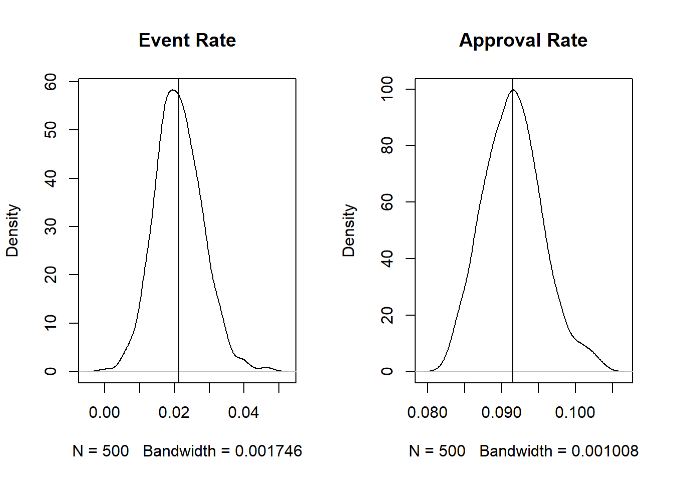
Based on the above simulations, when using the model trained on the entire population and using a threshold of >=689 the average simulated event rates and approval rates are close to the expected rates from before. But what if we use the model developed only on the known good population?
smple %>%
  filter(segment == "KG") %>%  ## Filter on known goods only
  mutate(pred = predict(mdl_kg, newdata = .),   ## Generate predictions
         score = scaling_func(pred),  ## Scale output
         total = n()) %>%
  arrange(pred) %>%
  mutate(rn = row_number(),
         c_bad_rate = cumsum(bad_flag)/rn) %>%
  filter(c_bad_rate <= 0.02) %>%
  summarise(approve_count = n(),
            total = mean(total),
            score_cutoff = min(score),
            bad_rate = sum(bad_flag)/n()) %>%
  mutate(approval_rate = approve_count / total)
##   approve_count total score_cutoff  bad_rate approval_rate
## 1           904  9178          696 0.0199115     0.0984964
# Simulate using the model built only on the known good population
generate_sim(mdl_kg, cutoff = 696)
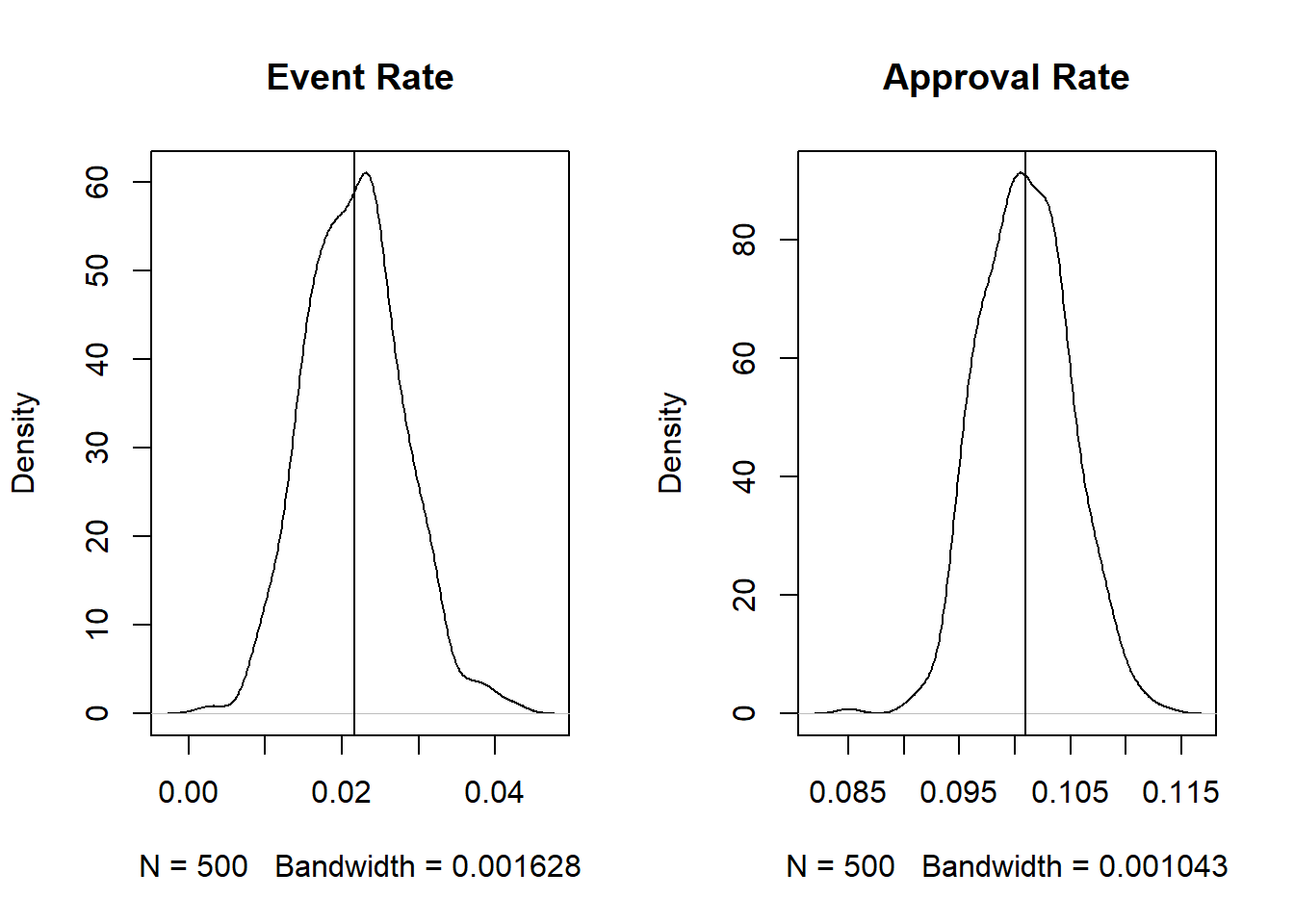
When using the known-good model, we can achieve a slightly higher approval rate keeping the event rate more or less the same. While the difference is not significant, a ~1% higher approval rate on a large funnel could be significant (psst. monthly targets anyone?).
While most modelers/data scientists understand this, explaining the need to build segmented models to a business owner can be easier if the impact can be linked to business outcomes 😉.
Thoughts? Comments? Helpful? Not helpful? Like to see anything else added in here? Let me know!