
This post is inspired by a really approachable post on particle swarm optimisation by Adrian Tam. We’ll build a basic particle swam optimiser in R and try to visualise the results.
Libraries
# install.packages(pacman)
pacman::p_load(dplyr, gganimate, metR)
Objective function
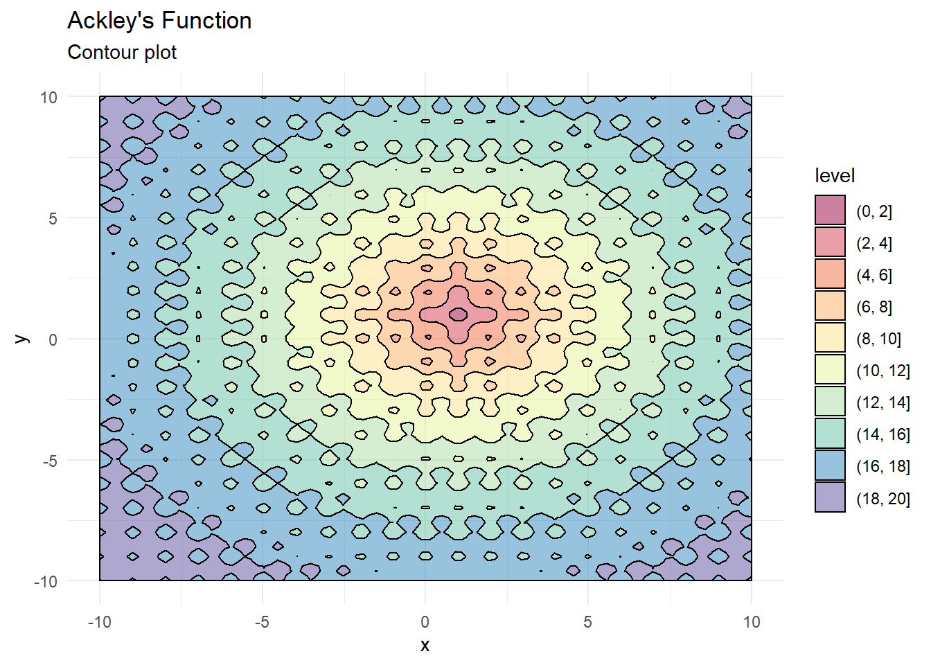
We’ll use the Ackley’s Function here to evaluate how well the optimiser works. The function has many local optima and should pose a challenge to the optimisation routine.
obj_func <- function(x, y){
  # Modifying for a different global minimum
  -20 * exp(-0.2 * sqrt(0.5 *((x-1)^2 + (y-1)^2))) - exp(0.5*(cos(2*pi*x) + cos(2*pi*y))) + exp(1) + 20
}
# Set of x and y values (search domain)
x <- seq(-10, 10, length.out = 100)
y <- seq(-10, 10, length.out = 100)

# Create a data frame that stores every permutation of
# x and y coordinates
grid <- expand.grid(x, y, stringsAsFactors = F)
head(grid)
##         Var1 Var2
## 1 -10.000000  -10
## 2  -9.797980  -10
## 3  -9.595960  -10
## 4  -9.393939  -10
## 5  -9.191919  -10
## 6  -8.989899  -10
# Evaluate the objective function at each x, y value
grid$z <- obj_func(grid[,1], grid[,2])

# create a contour plot
contour_plot <- ggplot(grid, aes(x = Var1, y = Var2)) +
  geom_contour_filled(aes(z = z), color = "black", alpha = 0.5) +
  scale_fill_brewer(palette = "Spectral") +
  theme_minimal() +
  labs(x = "x", y = "y", title = "Ackley's Function", subtitle = "Contour plot")

contour_plot
Optimiser basics
The optimiser works as such:
- Start with set of random search points uniformly distributed across the search domain
- Find the objective function value at each of these points
- Track the minimum(or maximum) value of the objective function achieved at each search point
- Move each search point a small amount in two directions:
- Towards the locally optimal value (for that point)
- Towards the globally optimal value (across all points)
- Repeat
Or to put it more formally:
Say we are operating in 2 dimensions (x and y coordinates). Then, for each particle i
$$x_{t+1}^i = x_{t}^i + \Delta{x_t}^i$$
$$y_{t+1}^i = y_{t}^i + \Delta{y_t}^i$$
And,
$$\Delta{x_t}^i = w\Delta{x_{t-1}^i} + c_1r_1(x_{localBest} - x_i) + c_2r_2(x_{globalBest} - x_i)$$
$$\Delta{y_t}^i = w\Delta{y_{t-1}^i} + c_1r_1(y_{localBest} - y_i) + c_2r_2(y_{globalBest} - y_i)$$
Where w, c1, c2, r1, r2 are positive constants. r1 and r2 are uniformly distributed (positive) random numbers. These random numbers need to be positive because the direction in which each particle will move is decided by where localBest and globalBest are. Again, localBest is the optimal function value observed by the ith particle and globalBest is the optimal function value across all particles.
Implementing a single iteration
Initial positions
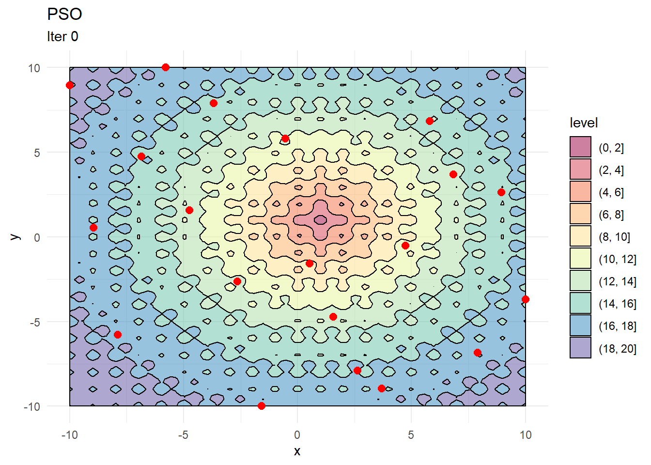
# Say we start with 20 particles
n_particles <- 20

# Set some initial values for constants
w <- 0.5
c1 <- 0.05
c2 <- 0.1

# Search domain in x and y coordinates
x <- seq(-10, 10, length.out = 20)
y <- seq(-10, 10, length.out = 20)

# Combine into a matrix
X <- data.frame(x = sample(x, n_particles, replace = F),
                y = sample(y, n_particles, replace = F))
# Chart starting locations
contour_plot +
  geom_point(data = X, aes(x, y), color = "red", size = 2.5) +
  labs(title = "PSO", subtitle = "Iter 0")
Starting perturbations
# Uniformly distributed (positive) perturbations
dX <- matrix(runif(n_particles * 2), ncol = 2)

# Scale down the perturbations by a factor (w in the equation above)
dX <- dX * w
# Set the location of the local best (optimal value) to starting positions
pbest <- X

# Evaluate the function at each point and store
pbest_obj <- obj_func(X[,1], X[,2])

# Find a global best and its position
gbest <- pbest[which.min(pbest_obj),]
gbest_obj <- min(pbest_obj)
X_dir <- X %>%
  mutate(g_x = gbest[1,1],
         g_y = gbest[1,2],
         angle = atan((g_y - y)/(g_x - x))*180/pi,
         angle = ifelse(g_x < x, 180 + angle, angle))

contour_plot +
  geom_point(data = X, aes(x, y), color = "red", size = 2.5) +
  geom_arrow(data = X_dir, aes(x, y, mag = 1, angle = angle), direction = "ccw", pivot = 0, show.legend = F) +
  labs(title = "PSO", subtitle = "Iter 0")

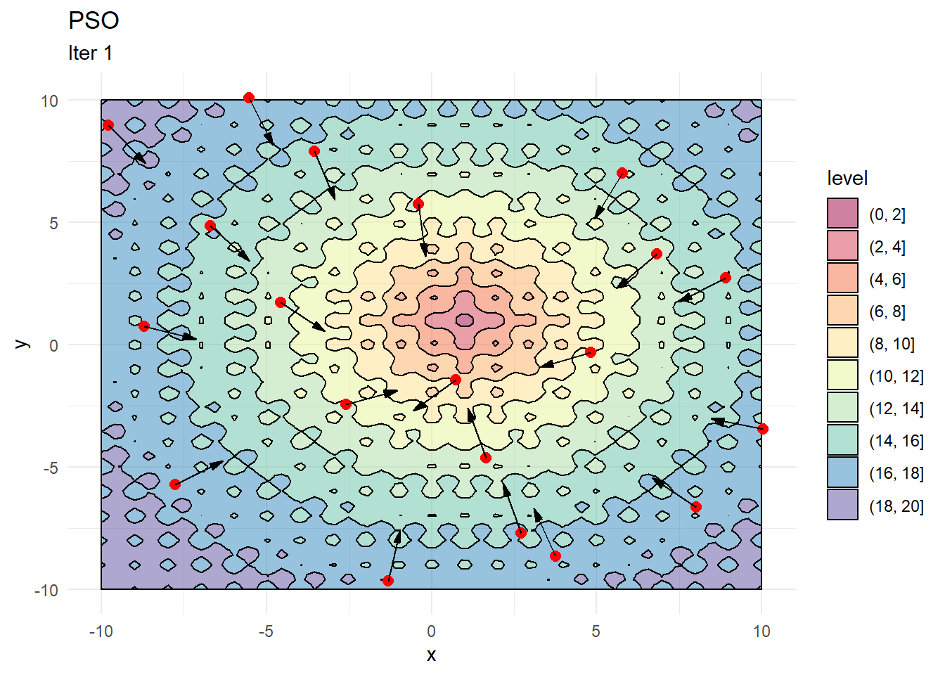
Updating Positions
# Update dx based on the equation shown previously
dX <- w * dX + c1*runif(1)*(pbest - X) + c2*runif(1)*(as.matrix(gbest) - X)

# Add dx to current locations
X <- X + dX

# Evaluate objective function at new positions
# Note that X[,1] is the first column i.e. x coordinates
obj <- obj_func(X[,1], X[,2])

# Find those points where the objective function is lower
# than previous iteration
idx <- which(obj >= pbest_obj)

# Update locations of local best and store local best values
pbest[idx,] <- X[idx,]
pbest_obj[idx] <- obj[idx]

# Identify the minimum value of the of the objective function
# amongst all points
idx <- which.min(pbest_obj)

# Store as global best
gbest <- pbest[idx,]
gbest_obj <- min(pbest_obj)
X_dir <- X %>%
  mutate(g_x = gbest[1,1],
         g_y = gbest[1,2],
         angle = atan((g_y - y)/(g_x - x))*180/pi, # Need angles to show direction
         angle = ifelse(g_x < x, 180 + angle, angle))

contour_plot +
  geom_point(data = X, aes(x, y), color = "red", size = 2.5) +
  geom_arrow(data = X_dir, aes(x, y, mag = 1, angle = angle), direction = "ccw", pivot = 0, show.legend = F) +
  labs(title = "PSO", subtitle = "Iter 1")
Putting it all together
We can now encapsulate everything inside a function for ease of use.
# Final function
pso_optim <- function(obj_func,  #Accept a function directly
                      c1 = 0.05,
                      c2 = 0.05,
                      w = 0.8,
                      n_particles = 20,
                      init_fact = 0.1,
                      n_iter = 50,
                      ...   # This ensures we can pass any additional
                            # parameters to the objective function
){

  x <- seq(min(x), max(x), length.out = 100)
  y <- seq(min(y), max(y), length.out = 100)

  X <- cbind(sample(x, n_particles, replace = F),
             sample(y, n_particles, replace = F))

  dX <- matrix(runif(n_particles * 2) * init_fact, ncol = 2)

  pbest <- X
  pbest_obj <- obj_func(x = X[,1], y = X[,2])

  gbest <- pbest[which.min(pbest_obj),]
  gbest_obj <- min(pbest_obj)

  loc_df <- data.frame(X, iter = 0)
  iter <- 1

  while(iter < n_iter){

    dX <- w * dX + c1*runif(1)*(pbest - X) + c2*runif(1)*t(gbest - t(X))
    X <- X + dX

    obj <- obj_func(x = X[,1], y = X[,2])

    idx <- which(obj <= pbest_obj)
    pbest[idx,] <- X[idx,]
    pbest_obj[idx] <- obj[idx]

    idx <- which.min(pbest_obj)
    gbest <- pbest[idx,]
    gbest_obj <- min(pbest_obj)

    # Update iteration
    iter <- iter + 1
    loc_df <- rbind(loc_df, data.frame(X, iter = iter))
  }

  lst <- list(X = loc_df, obj = gbest_obj, obj_loc = paste0(gbest, collapse = ","))
  return(lst)
}
# Test optimiser
out <- pso_optim(obj_func,
                 x = x,
                 y = y,
                 c1 = 0.01,
                 c2 = 0.05,
                 w = 0.5,
                 n_particles = 50,
                 init_fact = 0.1,
                 n_iter = 200)
# Global minimum is at (1,1)
out$obj_loc
## [1] "0.999970489653139,1.00001974997258"
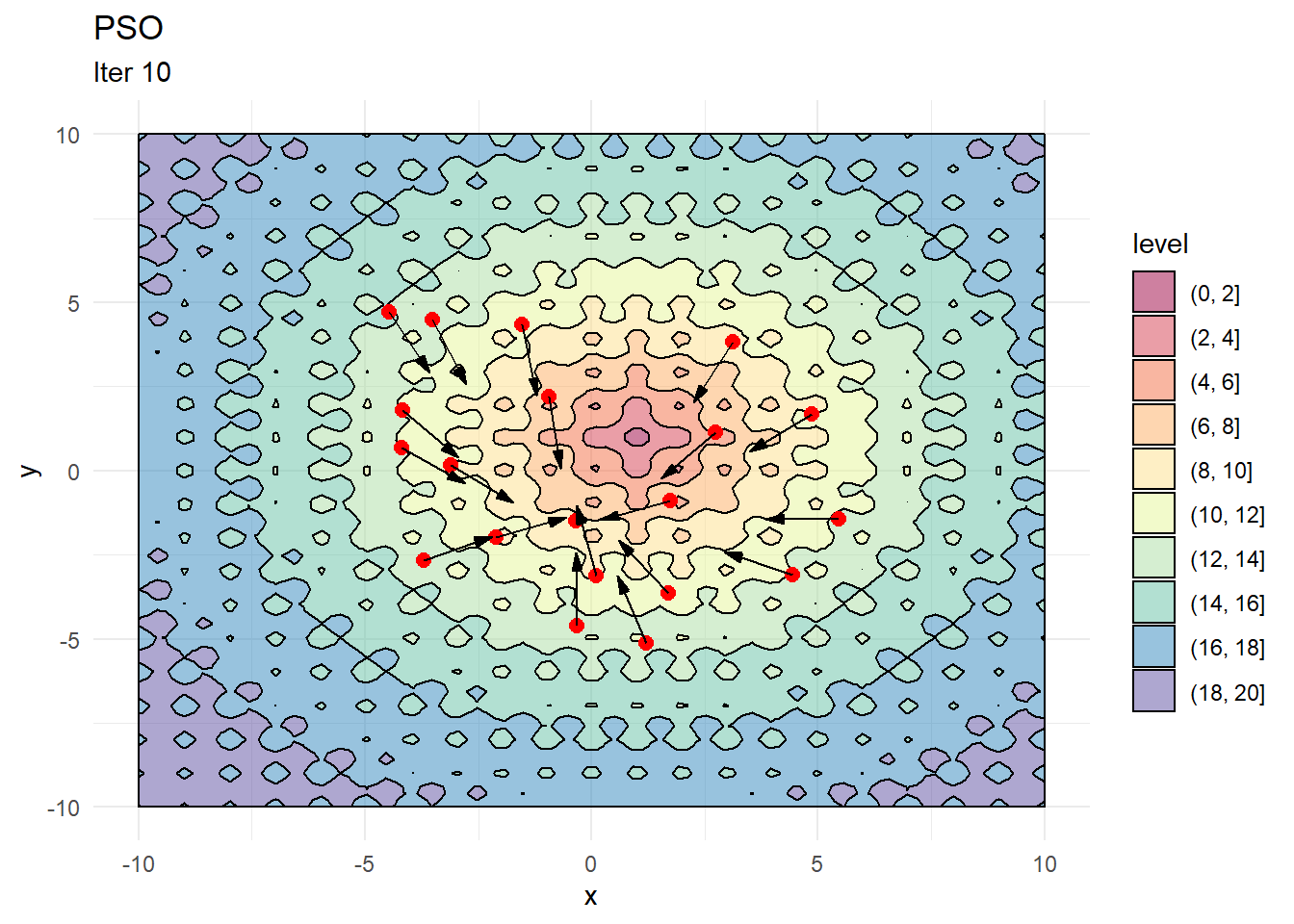
Animating results
This part is fun! We can use the awesome gganimate package to visualise the path of each point and see how the optimiser searches and converges towards an optimal value.
ggplot(out$X) +
  geom_contour(data = grid, aes(x = Var1, y = Var2, z = z), color = "black") +
  geom_point(aes(X1, X2)) +
  labs(x = "X", y = "Y") +
  transition_time(iter) +
  ease_aes("linear")
Parting notes
A few things are worth noting here:
c1decides how much a given point moves towards the best value that it has encountered thus far. Keeping this value low helps the optimiser converge faster.- Increasing
walso helps converge faster but if its too high and then the optimiser tends to swing back and forth between solutions.
Thoughts? Comments? Helpful? Not helpful? Like to see anything else added in here? Let me know!