Parallel Computing in R

performance

r-programming

Learn how to speed up your R code using parallel computing

Published

April 26, 2025

Packages

# Install packages if needed (uncomment to run)
# install.packages(c("parallel", "foreach", "doParallel", "tictoc"))

# Load the essential packages
library(parallel)    # Base R parallel functions
library(foreach)     # For parallel loops
library(doParallel)  # Backend for foreach
library(tictoc)      # For timing comparisons

Detecting Available CPU Cores

The first step involves checking how many CPU cores are available on the system:

# Detect the number of CPU cores
detectCores()

[1] 16

Good practice dictates leaving one core free for the operating system, so typically detectCores() - 1 is used for parallel operations.

The Basics

This section demonstrates creating a simple function that takes time to execute, then compares sequential versus parallel execution times:

# A function that takes time to execute
slow_function <- function(x) {
  Sys.sleep(0.5)  # Simulate computation time (half a second)
  return(x^2)     # Return the square of x
}

# Create a list of numbers to process
numbers <- 1:10

Method 1: Using parLapply (Works on All Systems)

This method works on all operating systems including Windows:

# Step 1: Create a cluster of workers
cl <- makeCluster(detectCores() - 1)

# Step 2: Export any functions our workers need
clusterExport(cl, "slow_function")

# Run the sequential version and time it
tic("Sequential version")
result_sequential <- lapply(numbers, slow_function)
toc()

Sequential version: 5.06 sec elapsed

# Run the parallel version and time it
tic("Parallel version")
result_parallel <- parLapply(cl, numbers, slow_function)
toc()

Parallel version: 0.52 sec elapsed

# Step 3: Always stop the cluster when finished!
stopCluster(cl)

# Verify both methods give the same results
all.equal(result_sequential, result_parallel)

[1] TRUE

Method 2: Using mclapply (Unix/Mac Only)

For Mac or Linux systems, this simpler approach can be utilized:

# For Mac/Linux users only
tic("Parallel mclapply (Mac/Linux only)")
result_parallel <- mclapply(numbers, slow_function, mc.cores = detectCores() - 1)
toc()

The foreach Package: A More Intuitive Approach

Many R practitioners find the foreach package easier to understand and implement. The package functions like a loop but can execute in parallel:

# Step 1: Create and register a parallel backend
cl <- makeCluster(detectCores() - 1)
registerDoParallel(cl)

# Run sequential foreach with %do%
tic("Sequential foreach")
result_sequential <- foreach(i = 1:10) %do% {
  slow_function(i)
}
toc()

Sequential foreach: 5.07 sec elapsed

# Run parallel foreach with %dopar%
tic("Parallel foreach")
result_parallel <- foreach(i = 1:10) %dopar% {
  slow_function(i)
}
toc()

Parallel foreach: 0.57 sec elapsed

# Always stop the cluster when finished
stopCluster(cl)

# Verify results
all.equal(result_sequential, result_parallel)

[1] TRUE

Combining Results with foreach

One notable feature of foreach is the ease with which results can be combined:

# Create and register a parallel backend
cl <- makeCluster(detectCores() - 1)
registerDoParallel(cl)

# Sum all results automatically with .combine='+'
tic("Parallel sum of squares")
total <- foreach(i = 1:100, .combine = '+') %dopar% {
  i^2
}
toc()

Parallel sum of squares: 0.11 sec elapsed

# Stop the cluster
stopCluster(cl)

# Verify the result
print(paste("Result obtained:", total))

[1] "Result obtained: 338350"

print(paste("Correct answer:", sum((1:100)^2)))

[1] "Correct answer: 338350"

Matrix Operations

Let’s try something more realistic. Matrix operations are perfect for parallelization:

# A more computationally intensive function
matrix_function <- function(n) {
  # Create a random n×n matrix
  m <- matrix(rnorm(n*n), ncol = n)
  # Calculate eigenvalues (computationally expensive)
  eigen(m)
  return(sum(diag(m)))
}

# Let's process 8 matrices of size 300×300
matrix_sizes <- rep(300, 8)

Performance Comparison

Let’s compare how different methods perform:

# Sequential execution
tic("Sequential")
sequential_result <- lapply(matrix_sizes, matrix_function)
sequential_time <- toc(quiet = TRUE)
sequential_time <- sequential_time$toc - sequential_time$tic

# Parallel with parLapply
cl <- makeCluster(detectCores() - 1)
clusterExport(cl, "matrix_function")
tic("parLapply")
parlapply_result <- parLapply(cl, matrix_sizes, matrix_function)
parlapply_time <- toc(quiet = TRUE)
parlapply_time <- parlapply_time$toc - parlapply_time$tic
stopCluster(cl)

# Parallel with foreach
cl <- makeCluster(detectCores() - 1)
registerDoParallel(cl)
tic("foreach")
foreach_result <- foreach(s = matrix_sizes) %dopar% {
  matrix_function(s)
}
foreach_time <- toc(quiet = TRUE)
foreach_time <- foreach_time$toc - foreach_time$tic
stopCluster(cl)

# Create a results table
results <- data.frame(
  Method = c("Sequential", "parLapply", "foreach"),
  Time = c(sequential_time, parlapply_time, foreach_time),
  Speedup = c(1, sequential_time/parlapply_time, sequential_time/foreach_time)
)

# Display the results
results

      Method Time  Speedup
1 Sequential 1.75 1.000000
2  parLapply 0.23 7.608696
3    foreach 0.23 7.608696

Visualizing Results

# Load ggplot2 for visualization
library(ggplot2)

# Plot execution times
ggplot(results, aes(x = reorder(Method, -Time), y = Time, fill = Method)) +
  geom_bar(stat = "identity") +
  labs(title = "Execution Time Comparison",
       x = "Method", y = "Time (seconds)") +
  theme_minimal() +
  theme(axis.text.x = element_text(angle = 45, hjust = 1))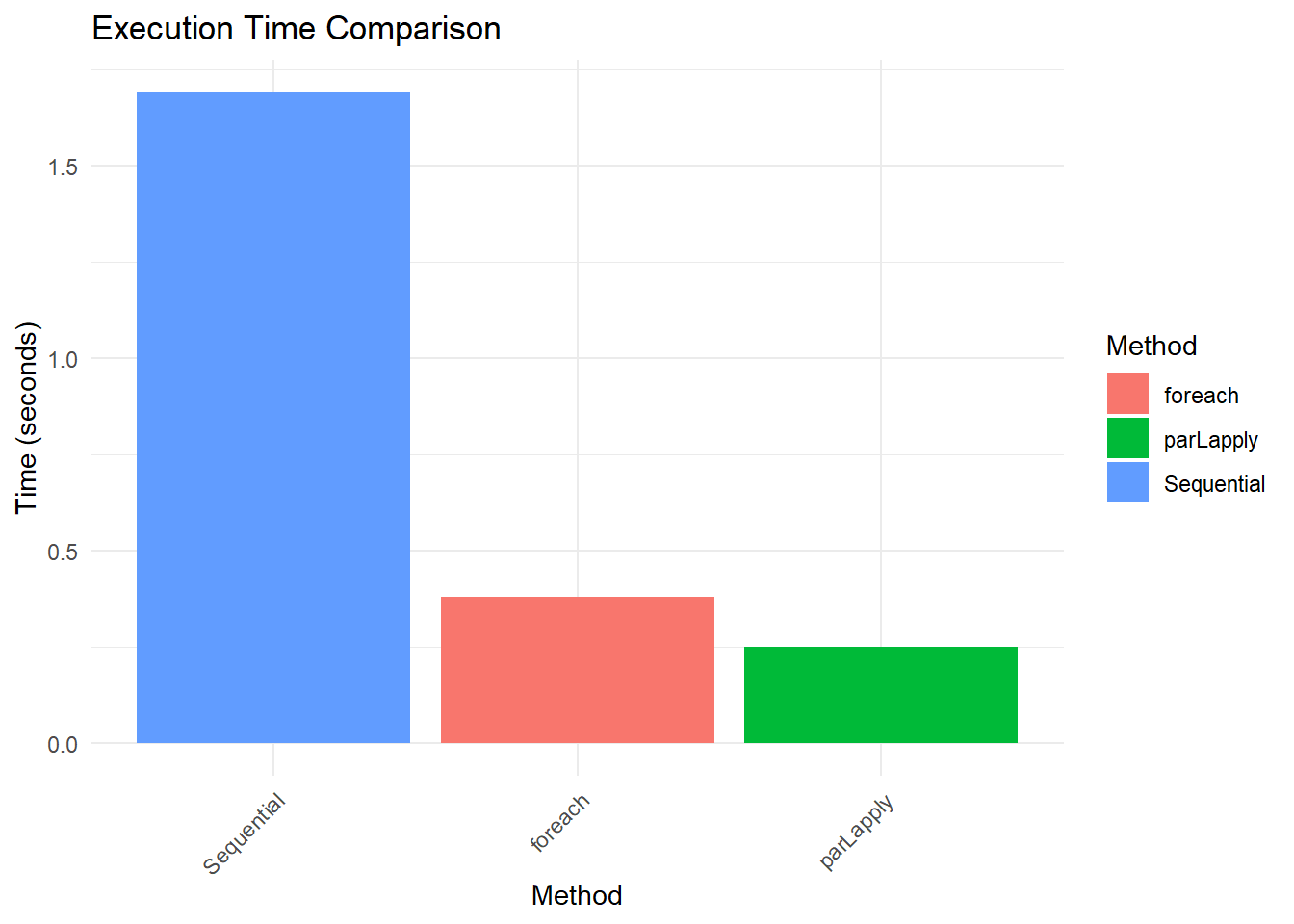

# Plot speedup
ggplot(results, aes(x = reorder(Method, Speedup), y = Speedup, fill = Method)) +
  geom_bar(stat = "identity") +
  labs(title = "Speedup Comparison",
       x = "Method", y = "Times faster than sequential") +
  theme_minimal() +
  theme(axis.text.x = element_text(angle = 45, hjust = 1))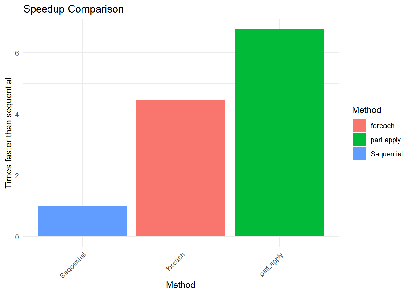

Practical Implementation

Parallel computing isn’t always the optimal choice. Here are some considerations:

✅ Good for parallelization: - Independent calculations (like applying the same function to different data chunks) - Computationally intensive tasks (simulations, bootstrap resampling) - Tasks that take more than a few seconds to run sequentially

❌ Not good for parallelization: - Very quick operations (parallelization overhead may exceed the time saved) - Tasks with heavy dependencies between steps - I/O-bound operations (reading/writing files)

Best Practices

Always stop clusters with stopCluster(cl) when processing is complete
Leave one core free for the operating system
Start small and test with a subset of data
Monitor memory usage - each worker needs its own copy of the data