# Load required packages
library(dplyr)     # For data manipulation
library(ggplot2)   # For visualization
library(gganimate) # For animations
library(metR) # For geom_arrowImplementing Particle Swarm Optimization from Scratch in R
R
Optimization
Visualization
Nature-inspired optimization algorithms can be surprisingly effective at navigating complex, high-dimensional search spaces. In this post, let’s build a Particle Swarm Optimization (PSO) algorithm from scratch in R.
Required Packages
Optimization Test Function: Ackley’s Function
Let’s use Ackley’s function as the benchmark — a challenging multimodal function with many local minima that trap conventional optimization algorithms:
obj_func <- function(x, y){
  # Modified Ackley function with global minimum at (1,1)
  -20 * exp(-0.2 * sqrt(0.5 *((x-1)^2 + (y-1)^2))) -
    exp(0.5*(cos(2*pi*x) + cos(2*pi*y))) + exp(1) + 20
}

# Create a visualization grid
x <- seq(-5, 5, length.out = 50)
y <- seq(-5, 5, length.out = 50)
grid <- expand.grid(x, y, stringsAsFactors = FALSE)
grid$z <- obj_func(grid[,1], grid[,2])

# Create a contour plot
contour_plot <- ggplot(grid, aes(x = Var1, y = Var2)) +
  geom_contour_filled(aes(z = z), color = "black", alpha = 0.5) +
  scale_fill_brewer(palette = "Spectral") +
  theme_minimal() +
  labs(x = "x", y = "y", title = "Ackley's Function")

contour_plot
Theoretical Foundation of Particle Swarm Optimization
PSO emulates the foraging behavior of biological swarms through individual memory and information sharing:
- Initialization: Random distribution of particles across the search space
- Memory Mechanism: Each particle maintains a record of its personal best position
- Information Sharing: The swarm collectively maintains knowledge of the global best position
- Movement Dynamics: Particles adjust their trajectories based on both personal experience and collective knowledge
The velocity update equation represents a balance of three fundamental forces:
\[v_{new} = w \cdot v_{current} + c_1 \cdot r_1 \cdot (p_{best} - p_{current}) + c_2 \cdot r_2 \cdot (g_{best} - p_{current})\]
Where:
w: Inertia (momentum preservation)c1: Personal influence (individual memory)c2: Social influence (collective cooperation)r1,r2: Stochastic components
Sample Implementation
Swarm Initialization
The initial phase involves creating a randomized swarm of particles and distributing them across the defined search space:
# Set parameters
n_particles <- 20
w <- 0.5     # Inertia weight
c1 <- 0.05   # Personal learning rate
c2 <- 0.1    # Social learning rate

# Create random particle positions
x_range <- seq(-5, 5, length.out = 20)
y_range <- seq(-5, 5, length.out = 20)
X <- data.frame(
  x = sample(x_range, n_particles, replace = FALSE),
  y = sample(y_range, n_particles, replace = FALSE)
)

# Visualize initial positions
contour_plot +
  geom_point(data = X, aes(x, y), color = "red", size = 2.5) +
  labs(title = "Initial Particle Positions")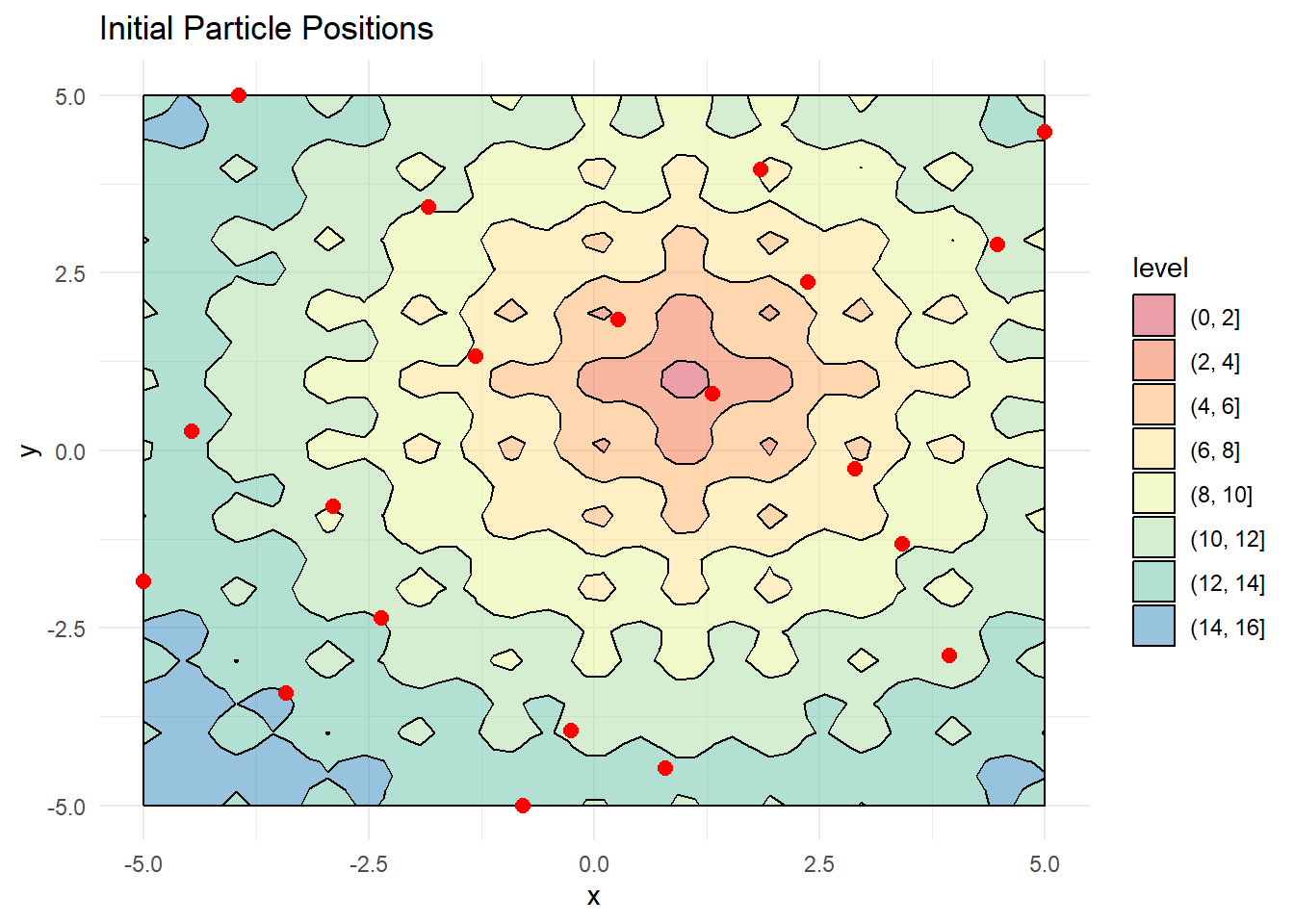
Global Best Position and Velocity Initialization
Next, we need to track each particle’s personal best position and the swarm’s global best position, while initializing velocity vectors:
# Initialize random velocities
dX <- matrix(runif(n_particles * 2), ncol = 2) * w

# Set initial personal best positions
pbest <- X
pbest_obj <- obj_func(X[,1], X[,2])

# Find global best position
gbest <- pbest[which.min(pbest_obj),]
gbest_obj <- min(pbest_obj)

# Visualize with arrows showing pull toward global best
X_dir <- X %>%
  mutate(g_x = gbest[1,1],
         g_y = gbest[1,2],
         angle = atan((g_y - y)/(g_x - x))*180/pi,
         angle = ifelse(g_x < x, 180 + angle, angle))

contour_plot +
  geom_point(data = X, aes(x, y), color = "red", size = 2.5) +
  geom_segment(data = X_dir,
               aes(x = x, y = y,
                   xend = x + 0.5*cos(angle*pi/180),
                   yend = y + 0.5*sin(angle*pi/180)),
               arrow = arrow(length = unit(0.1, "cm")),
               color = "blue") +   labs(title = "Forces Acting on Particles")
Position Update Mechanism
The position update process implements the core PSO algorithm, calculating new velocities based on the fundamental equation and updating particle positions accordingly:
# Calculate new velocities using PSO equation
dX <- w * dX +
      c1*runif(1)*(pbest - X) +
      c2*runif(1)*(as.matrix(gbest) - X)

# Update positions
X <- X + dX

# Evaluate function at new positions
obj <- obj_func(X[,1], X[,2])

# Update personal best positions if improved
idx <- which(obj <= pbest_obj)
pbest[idx,] <- X[idx,]
pbest_obj[idx] <- obj[idx]

# Update global best position
idx <- which.min(pbest_obj)
gbest <- pbest[idx,]
gbest_obj <- min(pbest_obj)

# Visualize updated positions
X_dir <- X %>%
  mutate(g_x = gbest[1,1],
         g_y = gbest[1,2],
         angle = atan((g_y - y)/(g_x - x))*180/pi,
         angle = ifelse(g_x < x, 180 + angle, angle))

contour_plot +
  geom_point(data = X, aes(x, y), color = "red", size = 2.5) +
  geom_segment(data = X_dir,
               aes(x = x, y = y,
                   xend = x + 0.5*cos(angle*pi/180),
                   yend = y + 0.5*sin(angle*pi/180)),
               arrow = arrow(length = unit(0.1, "cm")),
               color = "blue") +
  labs(title = "Particles After First Update")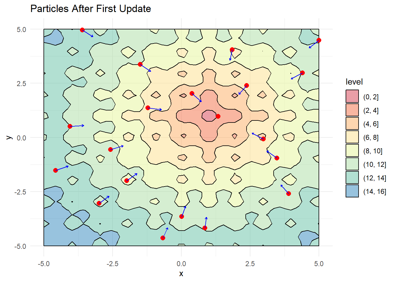
Full Implementation
The following implementation encapsulates the complete PSO algorithm within a reusable function framework:
pso_optim <- function(obj_func,      # Function to minimize
                      c1 = 0.05,      # Personal learning rate
                      c2 = 0.05,      # Social learning rate
                      w = 0.8,        # Inertia weight
                      n_particles = 20,  # Swarm size
                      init_fact = 0.1,   # Initial velocity factor
                      n_iter = 50        # Maximum iterations
){
  # Define search domain
  x <- seq(-5, 5, length.out = 100)
  y <- seq(-5, 5, length.out = 100)

  # Initialize particles
  X <- cbind(sample(x, n_particles, replace = FALSE),
             sample(y, n_particles, replace = FALSE))
  dX <- matrix(runif(n_particles * 2) * init_fact, ncol = 2)

  # Initialize best positions
  pbest <- X
  pbest_obj <- obj_func(x = X[,1], y = X[,2])
  gbest <- pbest[which.min(pbest_obj),]
  gbest_obj <- min(pbest_obj)

  # Store positions for visualization
  loc_df <- data.frame(X, iter = 0)
  iter <- 1

  # Main optimization loop
  while(iter < n_iter){
    # Update velocities
    dX <- w * dX +
          c1*runif(1)*(pbest - X) +
          c2*runif(1)*t(gbest - t(X))

    # Update positions
    X <- X + dX

    # Evaluate and update best positions
    obj <- obj_func(x = X[,1], y = X[,2])
    idx <- which(obj <= pbest_obj)
    pbest[idx,] <- X[idx,]
    pbest_obj[idx] <- obj[idx]

    # Update global best
    idx <- which.min(pbest_obj)
    gbest <- pbest[idx,]
    gbest_obj <- min(pbest_obj)

    # Store for visualization
    iter <- iter + 1
    loc_df <- rbind(loc_df, data.frame(X, iter = iter))
  }

  return(list(X = loc_df,
              obj = gbest_obj,
              obj_loc = paste0(gbest, collapse = ",")))
}
The following code snippet applies the PSO algorithm to the Ackley function:
# Run the PSO algorithm
out <- pso_optim(obj_func,
                 c1 = 0.01,    # Low personal influence
                 c2 = 0.05,    # Moderate social influence
                 w = 0.5,      # Medium inertia
                 n_particles = 50,
                 init_fact = 0.1,
                 n_iter = 200)

# Check the result (global minimum should be at (1,1))
out$obj_loc
[1] "0.999993503801879,1.00000730109038"Visualising Swarm Behavior
The optimization process can be effectively visualized through animation, demonstrating the collective convergence behavior of the particle swarm:
# Create animation of the optimization process
ggplot(out$X) +
  geom_contour(data = grid, aes(x = Var1, y = Var2, z = z), color = "black") +
  geom_point(aes(X1, X2)) +
  labs(x = "X", y = "Y") +
  transition_time(iter) +
  ease_aes("linear")
Parameter Optimization and Algorithm Tuning
The PSO algorithm’s performance characteristics can be substantially modified through systematic adjustment of three parameters:
- Inertia Weight (w)
- High values (>0.8): Particles maintain substantial momentum, aiding extensive exploration
- Low values (<0.4): Particles exhibit reduced momentum, facilitating solution refinement
- Personal Learning Rate (c1)
- High values: Particles prioritize individual discoveries and historical performance
- Low values: Particles demonstrate reduced reliance on personal experience
- Social Learning Rate (c2)
- High values: Particles demonstrate strong attraction toward the global optimum
- Low values: Particles maintain greater independence in exploration
Implementation Considerations
- Boundary Constraint Implementation: Enforce particle confinement within valid solution regions
- Adaptive Parameter Strategies: Implement dynamic parameter adjustment during optimization execution
- Convergence-Based Termination: Establish sophisticated stopping criteria based on solution convergence
- High-Dimensional Extension: Adapt the algorithm for complex, multi-dimensional optimization problems
The R package
psoprovides a comprehensive, production-ready implementation suitable for industrial applications.
Key Takeaways
- PSO successfully emulates biological swarm intelligence through mathematical modeling of collective behavior patterns
- The velocity update equation balances three critical forces: inertia, personal experience, and social influence
- Parameter tuning significantly affects algorithm performance, with distinct configurations optimizing exploration versus exploitation
- The algorithm scales effectively to high-dimensional problems while maintaining computational efficiency
- Production implementations require boundary constraints and adaptive parameters for robust performance