Generating Correlated Random Numbers in R Using Matrix Methods

Introduction

The generation of random data with specified correlation patterns can be useful in statistical simulation and this tutorial provides a methodology for creating correlated random numbers in R. The techniques presented enable the development of realistic synthetic datasets with precisely controlled correlation structures, essential for robust statistical analysis and model validation.

The Cholesky Decomposition Method

# Load required packages
library(ggplot2)
library(dplyr)

# 1. Define your target correlation matrix
cor_mat <- matrix(c(1, 0.3, 
                   0.3, 1), nrow = 2, byrow = TRUE)

# 2. Apply Cholesky decomposition
chol_mat <- chol(cor_mat)

# 3. Generate uncorrelated random numbers
old_random <- matrix(rnorm(2000), ncol = 2)

# 4. Transform to create correlation
new_random <- old_random %*% chol_mat

# Verify the correlation
cor(new_random)

          [,1]      [,2]
[1,] 1.0000000 0.2679134
[2,] 0.2679134 1.0000000

The resulting new_random matrix contains values exhibiting approximately the target correlation structure.

Implementation Considerations

Independence

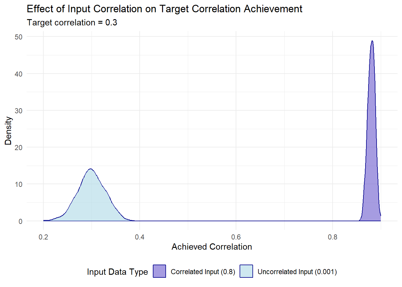
The input data must demonstrate statistical independence for the Cholesky method to function correctly. Pre-existing correlations in the input data compromise the method’s ability to achieve target correlation structures:

# What happens with already correlated input?
simulate_correlation <- function(input_correlation, target = 0.3) {
  results <- replicate(1000, {
    # Create input with specified correlation
    x <- rnorm(1000)
    y <- input_correlation * x + rnorm(1000, sd = sqrt(1 - input_correlation^2))
    
    # Apply our method
    old_random <- cbind(x, y)
    chol_mat <- chol(matrix(c(1, target, target, 1), ncol = 2))
    new_random <- old_random %*% chol_mat
    
    # Return resulting correlation
    cor(new_random)[1,2]
  })
  return(results)
}

# Compare results with different input correlations
correlated_results <- simulate_correlation(0.8, target = 0.3)
uncorrelated_results <- simulate_correlation(0.001, target = 0.3)

# Create data frame for ggplot2
plot_data <- data.frame(
  correlation = c(correlated_results, uncorrelated_results),
  input_type = factor(rep(c("Correlated Input (0.8)", "Uncorrelated Input (0.001)"), 
                         each = length(correlated_results)))
)

# Create density plot with ggplot2
ggplot(plot_data, aes(x = correlation, fill = input_type, color = input_type)) +
  geom_density(alpha = 0.6) +
  labs(title = "Effect of Input Correlation on Target Correlation Achievement",
       subtitle = "Target correlation = 0.3",
       x = "Achieved Correlation",
       y = "Density",
       fill = "Input Data Type",
       color = "Input Data Type") +
  theme_minimal() +
  theme(legend.position = "bottom") +
  scale_fill_manual(values = c("slateblue", "lightblue")) +
  scale_color_manual(values = c("darkblue", "darkblue"))

When input data contains pre-existing correlation patterns, the Cholesky method cannot effectively override these relationships to establish the desired target correlation structure.

Distribution Consistency

Optimal results require consistent probability distributions across all variables in the transformation:

# Different distributions cause problems
set.seed(123)
x1 <- rchisq(1000, df = 3)  # Chi-squared (skewed)
y1 <- rnorm(1000)           # Normal (symmetric)
old_mixed <- cbind(x1, y1)

# Same distribution works better
x2 <- rchisq(1000, df = 3)
y2 <- rchisq(1000, df = 3)
old_same <- cbind(x2, y2)

# Apply the same transformation to both
chol_mat <- chol(matrix(c(1, 0.7, 0.7, 1), ncol = 2))
new_mixed <- old_mixed %*% chol_mat
new_same <- old_same %*% chol_mat

# Compare results
cat("Target correlation: 0.7\n")

Target correlation: 0.7

cat("Mixed distributions result:", round(cor(new_mixed)[1,2], 3), "\n")

Mixed distributions result: 0.915 

cat("Same distribution result:", round(cor(new_same)[1,2], 3))

Same distribution result: 0.699

The combination of different probability distributions (such as normal and chi-squared) can result in unexpected correlation patterns following the Cholesky transformation.

Distribution Properties

The Cholesky transformation may fundamentally alter the statistical properties of the original data:

# Original positive-only distribution
x <- rchisq(1000, df = 3)  # Always positive
y <- rchisq(1000, df = 3)  # Always positive
old_random <- cbind(x, y)

# Apply negative correlation
chol_mat <- chol(matrix(c(1, -0.7, -0.7, 1), ncol = 2))
new_random <- old_random %*% chol_mat

# Check what happened
cat("Original data range:", round(range(old_random), 2), "\n")

Original data range: 0.02 19.93 

cat("Transformed data range:", round(range(new_random), 2), "\n")

Transformed data range: -12.81 19.93 

cat("Negative values in result:", sum(new_random < 0), "out of", length(new_random))

Negative values in result: 488 out of 2000

The Cholesky transformation can fundamentally modify data characteristics, such as introducing negative values into previously positive-only distributions, thereby altering the fundamental nature of the data.

Alternate Implementation: mvtnorm

For practical applications requiring efficient implementation, the mvtnorm package provides a streamlined solution for generating multivariate normal distributions with specified correlation structures:

# Load the package
library(mvtnorm)

# Define means and covariance matrix
means <- c(10, 20)  # Mean for each variable
sigma <- matrix(c(4, 2,   # Covariance matrix
                  2, 3), ncol = 2)

# See the implied correlation
cov2cor(sigma)

          [,1]      [,2]
[1,] 1.0000000 0.5773503
[2,] 0.5773503 1.0000000

# Generate correlated normal data in one step
x <- rmvnorm(n = 1000, mean = means, sigma = sigma)

# Verify the result
round(cor(x), 3)

      [,1]  [,2]
[1,] 1.000 0.613
[2,] 0.613 1.000

Key Takeaways

• Cholesky decomposition provides a mathematical foundation for transforming uncorrelated data into correlated structures through matrix operations
• Input data independence is critical for successful correlation induction; pre-existing correlations compromise the transformation effectiveness
• Distribution consistency across variables ensures optimal results and prevents unexpected correlation artifacts
• The transformation process can alter fundamental data properties, requiring careful consideration of distributional characteristics
• The mvtnorm package offers production-ready solutions for multivariate normal data generation with specified correlation structures
• Method selection depends on specific requirements: Cholesky for educational and custom applications, mvtnorm for operational efficiency