R is a powerful language built for data analysis and visualization. This post walks through practical examples of using R for real-world analytics tasks.
Exploring a Dataset
R comes with several built-in datasets perfect for practice. This example examines the mtcars dataset:
# Statistical summary of key variablessummary(mtcars[, c("mpg", "wt", "hp")])
      mpg              wt              hp
 Min.   :10.40   Min.   :1.513   Min.   : 52.0
 1st Qu.:15.43   1st Qu.:2.581   1st Qu.: 96.5
 Median :19.20   Median :3.325   Median :123.0
 Mean   :20.09   Mean   :3.217   Mean   :146.7
 3rd Qu.:22.80   3rd Qu.:3.610   3rd Qu.:180.0
 Max.   :33.90   Max.   :5.424   Max.   :335.0
The mtcars dataset contains information about 32 cars from Motor Trend magazine, including fuel efficiency (mpg), weight (wt), and horsepower (hp).
Data Visualization
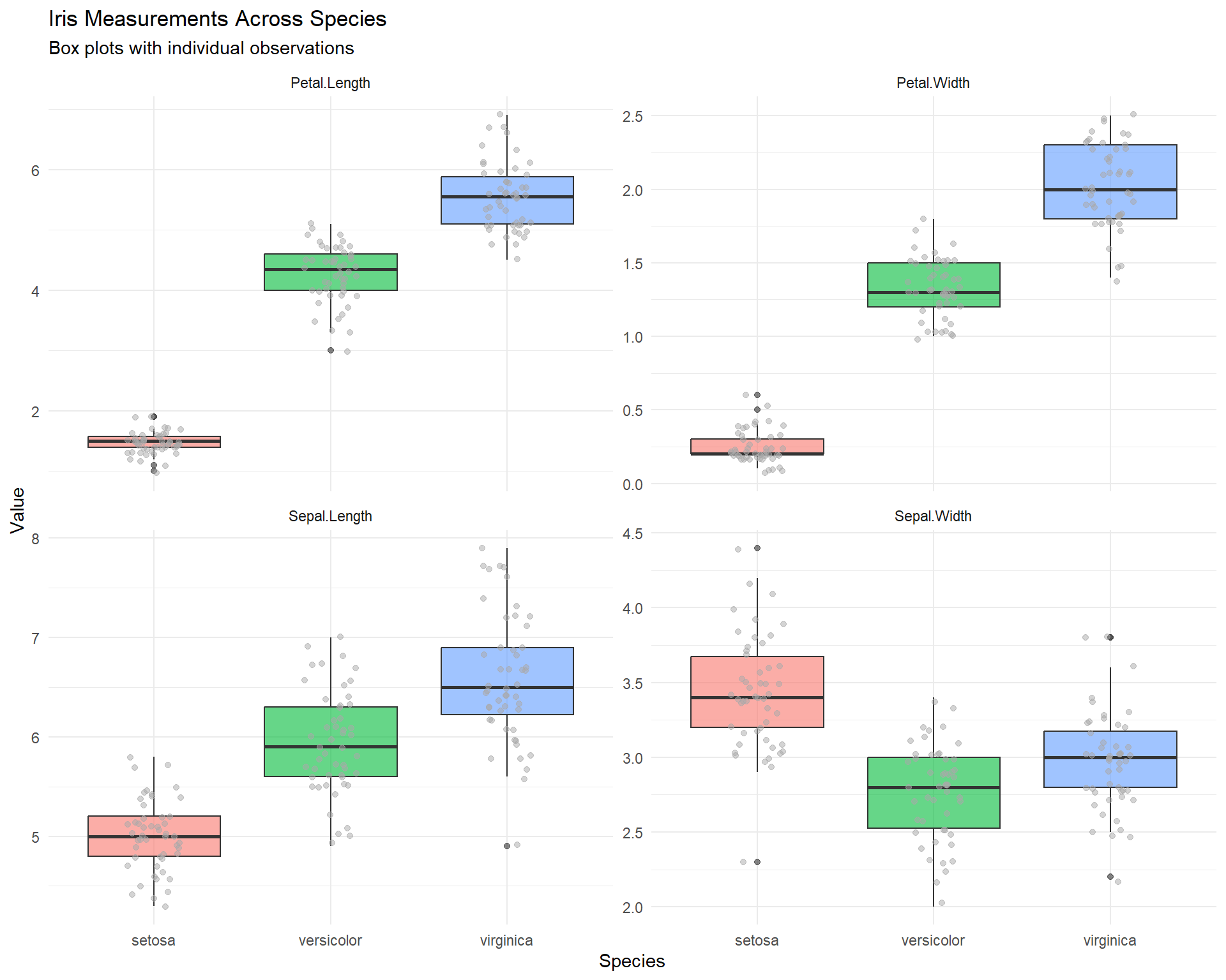
Visualization is essential for understanding patterns in data. The following examples create informative plots:
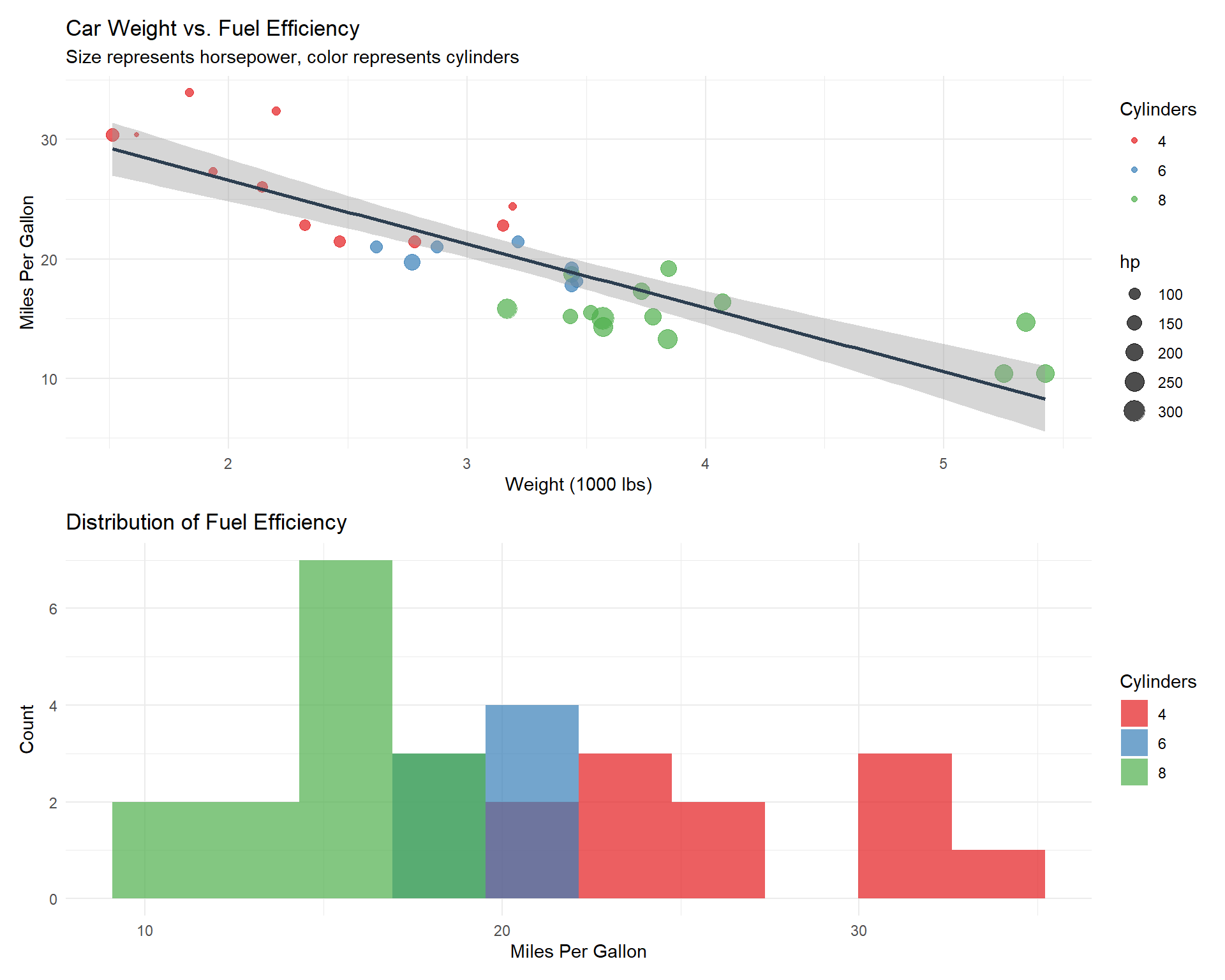
library(ggplot2)# 1. A scatter plot with regression linep1 <-ggplot(mtcars, aes(x = wt, y = mpg)) +geom_point(aes(size = hp, color =factor(cyl)), alpha =0.7) +geom_smooth(method ="lm", formula = y ~ x, color ="#2c3e50") +labs(title ="Car Weight vs. Fuel Efficiency",subtitle ="Size represents horsepower, color represents cylinders",x ="Weight (1000 lbs)",y ="Miles Per Gallon") +theme_minimal() +scale_color_brewer(palette ="Set1", name ="Cylinders")# 2. Distribution of fuel efficiencyp2 <-ggplot(mtcars, aes(x = mpg, fill =factor(cyl))) +geom_histogram(bins =10, alpha =0.7, position ="identity") +labs(title ="Distribution of Fuel Efficiency",x ="Miles Per Gallon",y ="Count") +scale_fill_brewer(palette ="Set1", name ="Cylinders") +theme_minimal()# Display plots (if using patchwork)library(patchwork)p1 / p2
These visualizations reveal:
A clear negative correlation between car weight and fuel efficiency
Higher cylinder cars tend to be heavier with lower MPG
The MPG distribution varies significantly by cylinder count
Data Transformation
Data rarely comes in the exact format needed. The dplyr package makes transformations straightforward:
# Load required packageslibrary(dplyr)library(tibble) # For rownames_to_column function# Create an enhanced version of the datasetmtcars_enhanced <- mtcars %>%# Add car names as a column (they're currently row names)rownames_to_column("car_name") %>%# Create useful derived metricsmutate(# Efficiency ratio (higher is better)efficiency_ratio = mpg / wt,# Power-to-weight ratio (higher is better)power_to_weight = hp / wt,# Categorize cars by efficiencyefficiency_category =case_when( mpg >25~"High Efficiency", mpg >15~"Medium Efficiency",TRUE~"Low Efficiency" ) ) %>%# Arrange from most to least efficientarrange(desc(efficiency_ratio))# Display the top 5 most efficient carshead(mtcars_enhanced[, c("car_name", "mpg", "wt", "hp", "efficiency_ratio", "efficiency_category")], 5)
        car_name  mpg    wt  hp efficiency_ratio efficiency_category
1   Lotus Europa 30.4 1.513 113         20.09253     High Efficiency
2    Honda Civic 30.4 1.615  52         18.82353     High Efficiency
3 Toyota Corolla 33.9 1.835  65         18.47411     High Efficiency
4       Fiat 128 32.4 2.200  66         14.72727     High Efficiency
5      Fiat X1-9 27.3 1.935  66         14.10853     High Efficiency
Answering Business Questions with Data
The enhanced dataset can be used to answer practical questions:
# Question 1: What are the average characteristics by cylinder count?cylinder_analysis <- mtcars_enhanced %>%group_by(cyl) %>%summarize(count =n(),avg_mpg =mean(mpg),avg_weight =mean(wt),avg_horsepower =mean(hp),avg_efficiency_ratio =mean(efficiency_ratio),avg_power_to_weight =mean(power_to_weight) ) %>%arrange(cyl)# Display the resultscylinder_analysis
customer_id age income years_as_customer
0 10 15 0
purchase_frequency
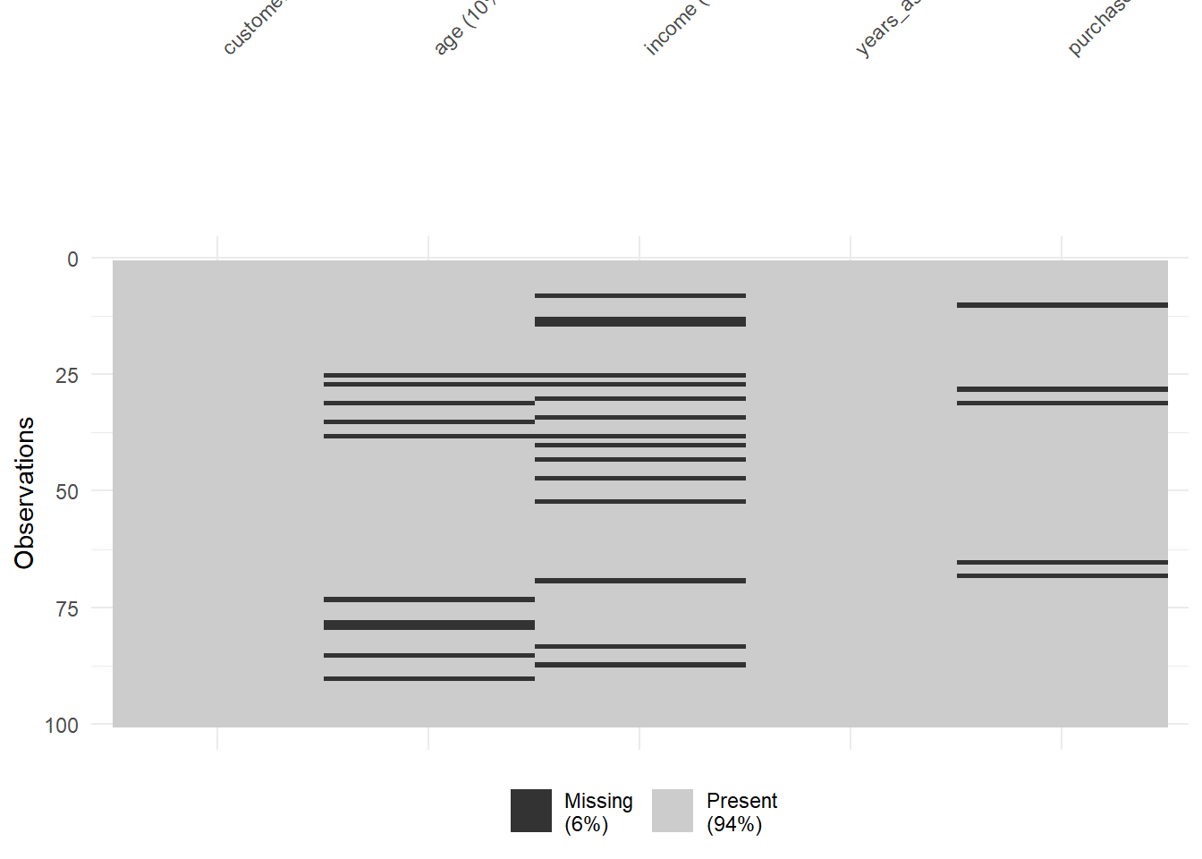
5
# 2. Visualize the pattern of missing datalibrary(naniar) # May need to install this packagevis_miss(customers)
# 3. Handle missing data with multiple approaches# Option A: Remove rows with any missing valuesclean_customers <-na.omit(customers)nrow(customers) -nrow(clean_customers) # Number of rows removed
[1] 26
# Option B: Impute with mean/median (numeric variables only)imputed_customers <- customers %>%mutate(age =ifelse(is.na(age), median(age, na.rm =TRUE), age),income =ifelse(is.na(income), mean(income, na.rm =TRUE), income),purchase_frequency =ifelse(is.na(purchase_frequency), median(purchase_frequency, na.rm =TRUE), purchase_frequency) )# Option C: Predictive imputation (using age to predict income)library(mice) # For more sophisticated imputation# Quick imputation model - in practice more parameters would be usedimputed_data <-mice(customers, m =5, method ="pmm", printFlag =FALSE)customers_complete <-complete(imputed_data)# Compare results by calculating customer value scorecalculate_value <-function(df) { df %>%mutate(customer_value = (income/10000) * (purchase_frequency/10) *log(years_as_customer +1)) %>%arrange(desc(customer_value)) %>%select(customer_id, customer_value, everything())}# Top 5 customers by value (original with NAs removed)head(calculate_value(clean_customers), 5)
Time series analysis is essential for understanding business trends and forecasting:
# Load packageslibrary(forecast)library(tseries)# Examine the built-in AirPassengers dataset (monthly air passengers from 1949 to 1960)data(AirPassengers)class(AirPassengers)
[1] "ts"
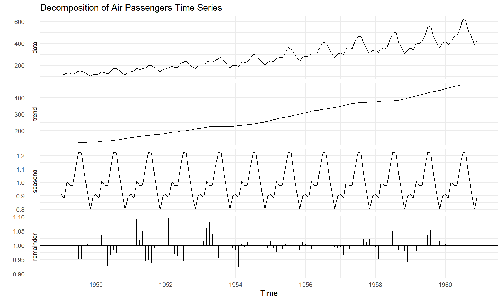
# Plot the time seriesautoplots <-autoplot(AirPassengers) +labs(title ="Monthly Air Passengers (1949-1960)",y ="Passenger Count",x ="Year") +theme_minimal()# Decompose the time series into seasonal componentsdecomposed <-decompose(AirPassengers, "multiplicative")autoplot(decomposed) +labs(title ="Decomposition of Air Passengers Time Series") +theme_minimal()
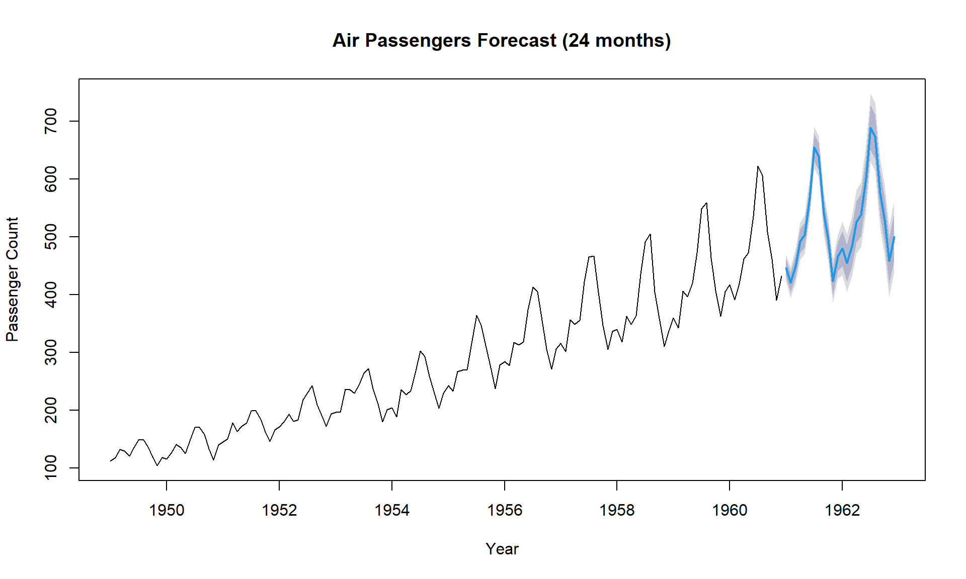
# Forecasting future values using auto.arimafit <-auto.arima(AirPassengers)forecasts <-forecast(fit, h =24) # Forecast 2 years ahead# Plot the forecastsplot(forecasts, main ="Air Passengers Forecast (24 months)",xlab ="Year", ylab ="Passenger Count")
# Summary of the forecast modelsummary(fit)
Series: AirPassengers
ARIMA(2,1,1)(0,1,0)[12]

Coefficients:
         ar1     ar2      ma1
      0.5960  0.2143  -0.9819
s.e.  0.0888  0.0880   0.0292

sigma^2 = 132.3:  log likelihood = -504.92
AIC=1017.85   AICc=1018.17   BIC=1029.35

Training set error measures:
                 ME     RMSE     MAE      MPE     MAPE     MASE        ACF1
Training set 1.3423 10.84619 7.86754 0.420698 2.800458 0.245628 -0.00124847