Monotonic Binning Using XGBoost

This post focuses on how to implement monotonic binning, a method that groups variable values into bins where event rates demonstrate consistent monotonic behavior. This methodology is essential in credit risk modeling, providing significant advantages in two critical areas:

1. Enhanced Model Stability: Monotonic relationships strengthen model robustness by reducing overfitting and ensuring reliable performance in production environments
2. Improved Interpretability: Monotonic constraints facilitate clear explanations by maintaining logical, consistent relationships between predictors and outcomes

Prerequisites and Required Libraries

library(recipes)  # For data preprocessing
library(dplyr)    # For data manipulation
library(xgboost)  # For creating monotonic bins
library(ggplot2)  # For visualization

Dataset Overview and Loading

This tutorial demonstrates the methodology using a sample from the Lending Club dataset, which provides comprehensive loan information including default indicators.

# Load sample data from Lending Club dataset
sample <- read.csv("https://bit.ly/42ypcnJ")

# Check dimensions of the dataset
dim(sample)

[1] 10000   153

Creating a Binary Target Variable

The first step involves constructing a binary target variable that clearly identifies loan defaults. This variable will serve as our outcome throughout the binning process:

# Define loan statuses that represent defaults
codes <- c("Charged Off", "Does not meet the credit policy. Status:Charged Off")

# Create binary target variable
model_data <- sample %>%
  mutate(bad_flag = ifelse(loan_status %in% codes, 1, 0))

Data Preprocessing

Before proceeding, the dataset must be prepared through systematic preprocessing. This step ensures data quality and compatibility with the XGBoost implementation. The process utilizes the recipes package to:

1. Filter and retain only numeric variables for analysis
2. Apply median imputation to handle missing values appropriately

# Create a recipe for preprocessing
rec <- recipe(bad_flag ~ ., data = model_data) %>%
  step_select(where(is.numeric)) %>%  # Keep only numeric variables
  step_impute_median(all_predictors())  # Fill missing values with medians

# Apply the preprocessing steps
rec <- prep(rec, training = model_data)
train <- bake(rec, new_data = model_data)

Step 3: Exploratory Analysis of Variable Relationships

It is crucial to examine the raw relationship between predictor variables and the target outcome. This analysis provides insights into underlying data patterns and validates the need for monotonic transformation.

This example analyzes the relationship between credit inquiries in the past 6 months and default rates:

# Create dataframe with inquiries and default flag
data.frame(x = model_data$inq_last_6mths,
           y = model_data$bad_flag) %>%
  filter(x <= 5) %>%  # Focus on 0-5 inquiries for clarity
  group_by(x) %>% 
  summarise(count = n(),  # Count observations in each group
            events = sum(y)) %>%  # Count defaults in each group
  mutate(pct = events/count) %>%  # Calculate default rate
  ggplot(aes(x = factor(x), y = pct)) + 
  geom_col() + 
  theme_minimal() + 
  labs(x = "# of inquiries in past 6 months", 
       y = "Default rate",
       title = "Default rate vs number of inquiries")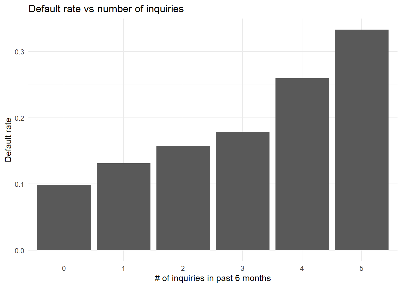

While the data exhibits a general upward trend (indicating that increased inquiries correlate with higher default rates), the relationship lacks perfect monotonicity. This validates the necessity of the monotonic binning approach to establish consistent patterns.

Implementing Monotonic Binning with XGBoost

The implementation uses XGBoost’s monotonicity constraints which enforces the model to generate splits that preserve a monotonic relationship with the target variable:

# Train XGBoost model with monotonicity constraint
mdl <- xgboost(
  data = train %>%
    select(inq_last_6mths) %>%  # Use only the inquiries variable
    as.matrix(),  
  label = train[["bad_flag"]],  # Target variable
  nrounds = 5,  # Number of boosting rounds
  params = list(
    booster = "gbtree",
    objective = "binary:logistic",
    monotone_constraints = 1,  # Force positive relationship
    max_depth = 1  # Simple trees with single splits
  ),
  verbose = 0  # Suppress output
)

Extracting Split Points and Constructing Final Bins

Following model training, the process extracts the optimal split points identified by XGBoost and utilizes them to construct the final bin structure:

# Extract split points from the model
splits <- xgb.model.dt.tree(model = mdl)  

# Create bin boundaries including -Inf and Inf for complete coverage
cuts <- c(-Inf, unique(sort(splits$Split)), Inf)

# Create and visualize the monotonic bins
data.frame(target = train$bad_flag,
           buckets = cut(train$inq_last_6mths, 
                         breaks = cuts, 
                         include.lowest = TRUE, 
                         right = TRUE)) %>% 
  group_by(buckets) %>%
  summarise(total = n(),  # Count observations in each bin
            events = sum(target == 1)) %>%  # Count defaults in each bin
  mutate(pct = events/total) %>%  # Calculate default rate
  ggplot(aes(x = buckets, y = pct)) + 
  geom_col() + 
  theme_minimal() + 
  labs(x = "Bins", 
       y = "Default rate",
       title = "Monotonic Bins for Inquiries")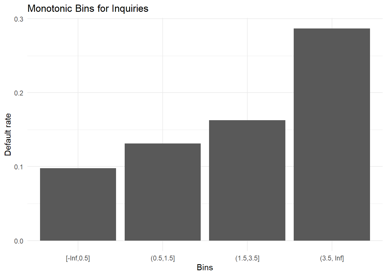

The default rates now demonstrate perfect monotonic behavior across all bins, creating a clearer and more interpretable relationship compared to the raw data.

Generalised Function

To enable implementation across multiple variables, a reusable function that encapsulates the entire monotonic binning workflow would be very useful here. Note the use of ranked correlation to identify the appropriate direction to be used inside the Xgboost call.

create_bins <- function(var, outcome, max_depth = 10, plot = TRUE){
  # Determine relationship direction automatically
  corr <- cor(var, outcome, method = "spearman")
  direction <- ifelse(corr > 0, 1, -1)  # 1 for positive, -1 for negative correlation
  
  # Build XGBoost model with appropriate monotonicity constraint
  mdl <- xgboost(
    verbose = 0,
    data = as.matrix(var),
    label = outcome,
    nrounds = 100,  # Single round is sufficient for binning
    params = list(objective = "binary:logistic",
                  monotone_constraints = direction,  # Apply constraint based on correlation
                  max_depth = max_depth))  # Control tree complexity
  
  # Extract and return split points
  splits <- xgb.model.dt.tree(model = mdl)
  cuts <- c(-Inf, sort(unique(splits$Split)), Inf)  # Include boundaries for complete coverage
  
  # Optionally visualize the bins
  if(plot) {
    data.frame(target = outcome,
               buckets = cut(var, 
                            breaks = cuts, 
                            include.lowest = TRUE, 
                            right = TRUE)) %>% 
      group_by(buckets) %>%
      summarise(total = n(),
                events = sum(target == 1)) %>%
      mutate(pct = events/total) %>%
      ggplot(aes(x = buckets, y = pct)) + 
      geom_col() + 
      theme_minimal() + 
      labs(x = "Bins", 
           y = "Default rate",
           title = "Monotonic Bins")
  }
  
  return(cuts)  # Return the bin boundaries
}

# Example: Create monotonic bins for annual income
income_bins <- create_bins(
  var = train$annual_inc,
  outcome = train$bad_flag,
  max_depth = 5
)