# install.packages("torch")
# torch::install_torch()Building a Simple Neural Network in R with torch
R
Deep Learning
torch
The torch package brings PyTorch to R. In this post, let’s build and train a simple neural network from scratch.
Installation
library(torch)
library(ggplot2)
A Simple Neural Network
This section focuses on the creation of a neural network to perform a simple regression task.
1. Sample Data
# Set seed for reproducibility
set.seed(42)

# Generate training data: y = 3x + 2 + noise
x <- torch_randn(100, 1)
y <- 3 * x + 2 + torch_randn(100, 1) * 0.3

# Display the first few data points
head(
  data.frame(
    x = as.numeric(x$squeeze()),
    y = as.numeric(y$squeeze())
  ))
x y
1 0.2753801 2.789203
2 0.7976708 4.444763
3 -2.5292332 -5.217783
4 -0.1811077 1.313051
5 -2.1584542 -4.372156
6 0.1204314 2.0149522. Neural Network Module
The next step involves defining the neural network architecture using torch’s module system:
# Define a simple feedforward neural network
nnet <- nn_module(
  initialize = function() {
    # Define layers
    self$layer1 <- nn_linear(1, 8)  # Input layer to hidden layer (1 -> 8 neurons)
    self$layer2 <- nn_linear(8, 1)  # Hidden layer to output layer (8 -> 1 neuron)
  },
  forward = function(x) {
    # Define forward pass
    x %>%
      self$layer1() %>%     # First linear transformation
      nnf_relu() %>%     # ReLU activation function
      self$layer2()         # Second linear transformation
  }
)

# Instantiate the model
model <- nnet()

# Display model structure
print(model)
An `nn_module` containing 25 parameters.
── Modules ─────────────────────────────────────────────────────────────────────
• layer1: <nn_linear> #16 parameters
• layer2: <nn_linear> #9 parameters3. Set Up the Optimizer and Loss Function
The training process requires defining how the model will learn from the data:
# Set up optimizer (Adam optimizer with learning rate 0.02)
optimizer <- optim_adam(model$parameters, lr = 0.02)

# Define loss function (Mean Squared Error for regression)
loss_fn <- nnf_mse_loss
4. Training Loop
The neural network training process proceeds as follows:
# Store loss values for plotting
loss_history <- numeric(300)

# Training loop
for(epoch in 1:300) {

  # Set model to training mode
  model$train()

  # Reset gradients
  optimizer$zero_grad()

  # Forward pass
  y_pred <- model(x)

  # Calculate loss
  loss <- loss_fn(y_pred, y)

  # Backward pass
  loss$backward()

  # Update parameters
  optimizer$step()

  # Store loss for plotting
  loss_history[epoch] <- loss$item()
}
5. Visualize the Training Progress
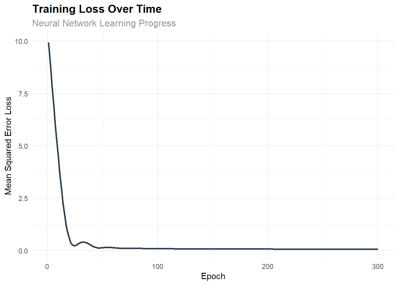
The following visualization demonstrates how the loss decreased during training:
# Create a data frame for plotting
training_df <- data.frame(
  epoch = 1:300,
  loss = loss_history
)

# Plot training loss
ggplot(training_df, aes(x = epoch, y = loss)) +
  geom_line(color = "#2c3e50", size = 1) +
  labs(
    title = "Training Loss Over Time",
    subtitle = "Neural Network Learning Progress",
    x = "Epoch",
    y = "Mean Squared Error Loss"
  ) +
  theme_minimal() +
  theme(
    plot.title = element_text(size = 14, face = "bold"),
    plot.subtitle = element_text(size = 12, color = "gray60")
  )
6. Visualize the Results
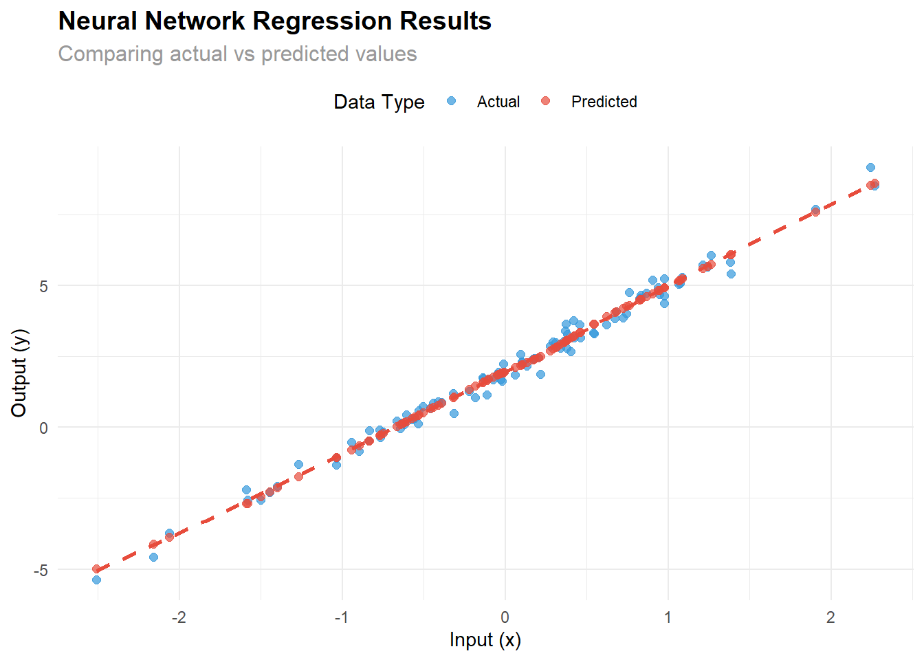
The following analysis demonstrates how well the trained model performs:
# Set model to evaluation mode
model$eval()

# Generate predictions
with_no_grad({
  y_pred <- model(x)
})

# Convert to R vectors for plotting
x_np <- as.numeric(x$squeeze())
y_np <- as.numeric(y$squeeze())
y_pred_np <- as.numeric(y_pred$squeeze())

# Create data frame for ggplot
plot_df <- data.frame(
  x = x_np,
  y_actual = y_np,
  y_predicted = y_pred_np
)

# Create the plot
ggplot(plot_df, aes(x = x)) +
  geom_point(aes(y = y_actual, color = "Actual"), alpha = 0.7, size = 2) +
  geom_point(aes(y = y_predicted, color = "Predicted"), alpha = 0.7, size = 2) +
  geom_smooth(aes(y = y_predicted), method = "loess", se = FALSE,
              color = "#e74c3c", linetype = "dashed") +
  labs(
    title = "Neural Network Regression Results",
    subtitle = "Comparing actual vs predicted values",
    x = "Input (x)",
    y = "Output (y)",
    color = "Data Type"
  ) +
  scale_color_manual(values = c("Actual" = "#3498db", "Predicted" = "#e74c3c")) +
  theme_minimal() +
  theme(
    plot.title = element_text(size = 14, face = "bold"),
    plot.subtitle = element_text(size = 12, color = "gray60"),
    legend.position = "top"
  )
7. Model Performance Analysis
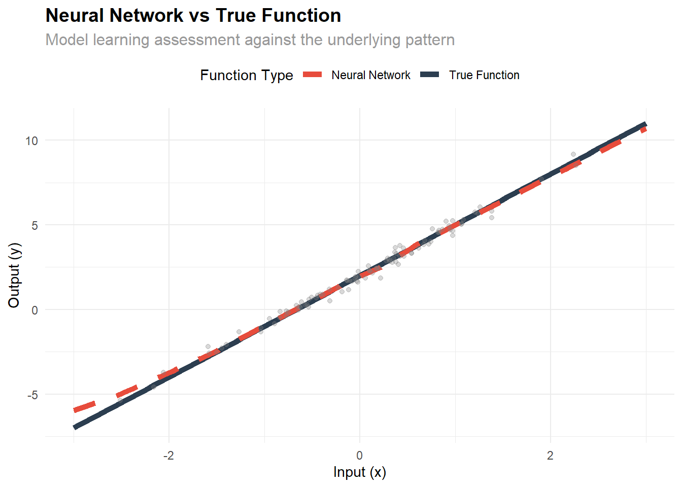
The following analysis examines how well the model learned the underlying pattern:
# Calculate performance metrics
mse <- mean((y_pred_np - y_np)^2)
rmse <- sqrt(mse)
mae <- mean(abs(y_pred_np - y_np))
r_squared <- cor(y_pred_np, y_np)^2

# Create performance summary
performance_summary <- data.frame(
  Metric = c("Mean Squared Error", "Root Mean Squared Error",
             "Mean Absolute Error", "R-squared"),
  Value = c(mse, rmse, mae, r_squared)
)

print(performance_summary)
Metric Value
1 Mean Squared Error 0.09108387
2 Root Mean Squared Error 0.30180104
3 Mean Absolute Error 0.22912676
4 R-squared 0.99159464# Compare with true relationship (y = 3x + 2)
# Generate predictions on a grid for comparison
x_grid <- torch_linspace(-3, 3, 100)$unsqueeze(2)
with_no_grad({
y_grid_pred <- model(x_grid)
})
x_grid_np <- as.numeric(x_grid$squeeze())
y_grid_pred_np <- as.numeric(y_grid_pred$squeeze())
y_grid_true <- 3 * x_grid_np + 2
# Plot comparison
comparison_df <- data.frame(
x = x_grid_np,
y_true = y_grid_true,
y_predicted = y_grid_pred_np
)
ggplot(comparison_df, aes(x = x)) +
geom_line(aes(y = y_true, color = "True Function"), size = 2) +
geom_line(aes(y = y_predicted, color = "Neural Network"), size = 2, linetype = "dashed") +
geom_point(data = plot_df, aes(y = y_actual), alpha = 0.3, color = "gray50") + labs(
title = "Neural Network vs True Function",
subtitle = "Model learning assessment against the underlying pattern",
x = "Input (x)",
y = "Output (y)",
color = "Function Type"
) +
scale_color_manual(values = c("True Function" = "#2c3e50", "Neural Network" = "#e74c3c")) +
theme_minimal() +
theme(
plot.title = element_text(size = 14, face = "bold"),
plot.subtitle = element_text(size = 12, color = "gray60"),
legend.position = "top"
)
Understanding the Neural Network
The following examination reveals what the network learned by analyzing its parameters:
# Extract learned parameters
layer1_weight <- as.matrix(model$layer1$weight$detach())
layer1_bias <- as.numeric(model$layer1$bias$detach())
layer2_weight <- as.matrix(model$layer2$weight$detach())
layer2_bias <- as.numeric(model$layer1$bias$detach())

cat("First layer (fc1) parameters:\n")
First layer (fc1) parameters:cat("Weight matrix shape:", dim(layer1_weight), "\n")Weight matrix shape: 8 1 cat("Bias vector length:", length(layer1_bias), "\n\n")Bias vector length: 8 cat("Second layer (fc2) parameters:\n")Second layer (fc2) parameters:cat("Weight matrix shape:", dim(layer2_weight), "\n")Weight matrix shape: 1 8 cat("Bias value:", layer2_bias, "\n\n")Bias value: -0.3651265 1.511045 -0.8437909 -0.4790628 0.1560887 -0.8598965 -0.1695607 0.1507583 # Display first layer weights and biases
cat("First layer weights:\n")First layer weights:print(round(layer1_weight, 4)) [,1]
[1,] -0.5380
[2,] 1.1316
[3,] -0.0922
[4,] -1.7453
[5,] 1.1420
[6,] 0.2002
[7,] 1.3589
[8,] -0.9909cat("\nFirst layer biases:\n")
First layer biases:print(round(layer2_bias, 4))[1] -0.3651 1.5110 -0.8438 -0.4791 0.1561 -0.8599 -0.1696 0.1508Experimenting with Different Architectures
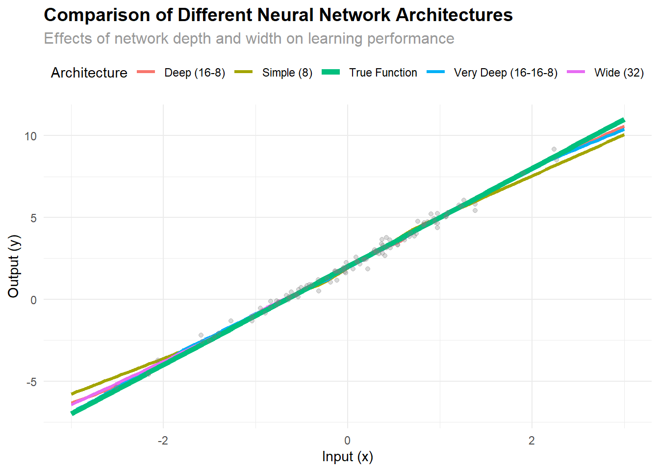
The following section analyzes the simple network against different architectures:
# Define different network architectures
create_network <- function(hidden_sizes) {
  nn_module(
    initialize = function(hidden_sizes) {
      self$layers <- nn_module_list()

      # Input layer
      prev_size <- 1

      for(i in seq_along(hidden_sizes)) {
        self$layers$append(nn_linear(prev_size, hidden_sizes[i]))
        prev_size <- hidden_sizes[i]
      }
      # Output layer
      self$layers$append(nn_linear(prev_size, 1))
    },
    forward = function(x) {
      for(i in 1:(length(self$layers) - 1)) {
        x <- nnf_relu(self$layers[[i]](x))
      }
      # No activation on output layer
      self$layers[[length(self$layers)]](x)
    }
  )
}

# Train different architectures
architectures <- list(
  "Simple (8)" = c(8),
  "Deep (16-8)" = c(16, 8),
  "Wide (32)" = c(32),
  "Very Deep (16-16-8)" = c(16, 16, 8)
)

results <- list()

for(arch_name in names(architectures)) {

  # Create and train model
  net_class <- create_network(architectures[[arch_name]])
  model_temp <- net_class(architectures[[arch_name]])
  optimizer_temp <- optim_adam(model_temp$parameters, lr = 0.01)

  # Quick training (fewer epochs for comparison)
  for(epoch in 1:200) {
    model_temp$train()
    optimizer_temp$zero_grad()
    y_pred_temp <- model_temp(x)
    loss_temp <- loss_fn(y_pred_temp, y)
    loss_temp$backward()
    optimizer_temp$step()
  }

  # Generate predictions
  model_temp$eval()
  with_no_grad({
    y_pred_arch <- model_temp(x_grid)
  })

  results[[arch_name]] <- data.frame(
    x = x_grid_np,
    y_pred = as.numeric(y_pred_arch$squeeze()),
    architecture = arch_name
  )
}

# Combine results
all_results <- do.call(rbind, results)

# Plot comparison
ggplot(all_results, aes(x = x, y = y_pred, color = architecture)) +
  geom_line(size = 1.2) +
  geom_line(data = comparison_df, aes(y = y_true, color = "True Function"),
            size = 2, linetype = "solid") +
  geom_point(data = plot_df, aes(x = x, y = y_actual),
             color = "gray50", alpha = 0.3, inherit.aes = FALSE) +  labs(
               title = "Comparison of Different Neural Network Architectures",
               subtitle = "Effects of network depth and width on learning performance",
               x = "Input (x)",
               y = "Output (y)",
               color = "Architecture"
             ) +
  theme_minimal() +
  theme(
    plot.title = element_text(size = 14, face = "bold"),
    plot.subtitle = element_text(size = 12, color = "gray60"),
    legend.position = "top"
  )
Key Takeaways
- Simple Architecture: Even a simple 2-layer network can learn complex patterns effectively
- Training Process: The importance of proper training loops with gradient computation
- Visualization: Effective methods for visualizing both training progress and results
- Model Evaluation: Understanding model performance through multiple metrics
- Architecture Comparison: How different network structures affect learning capabilities
The torch package provides a straightforward approach to building and experimenting with neural networks in R, bringing the power of deep learning to the R ecosystem. This approach can be extended to more complex datasets and deeper architectures as needed.