# install.packages(c("ragnar", "ellmer", "dplyr", "ggplot2", "tibble"))
library(ragnar)
library(ellmer)
library(dplyr)
library(ggplot2)
library(tibble)Text Analytics in R: Dense embeddings and RAG pipeline with ragnar and ellmer
R
NLP
RAG
LLMs
ragnar
ellmer
Required Packages
This earlier post explored building a text analytics pipeline using quanteda. We created a Document Feature Matrix (DFM), weighted it with TF-IDF, and measured document similarity using cosine similarity.
It worked, but we also ran into a limitation - cosine similarity alone might not be enough since the top most similar document did not match the document's sentiment
The root cause is not cosine similarity but the fact that we are measuring the cosine similarity of sparse TF-IDF vectors that encode word overlap, not meaning.
As an example, consider these sentences:
- “The borrower defaulted on their loan obligations.”
- “The client failed to meet repayment commitments.”
After stopword removal, they share zero vocabulary, producing near-zero TF-IDF cosine similarity. However, any analyst would consider these sentences semantically identical.
One fix is to use dense embeddings - neural representations where similar meanings map to nearby vectors. With dense embeddings, we should be able to capture semantic similarity between two sentences, even when they share no words.
In this post, let’s build a Retrieval Augmented Generation (RAG) pipeline in R using ragnar and ellmer to demonstrate the power of dense embeddings for retrieval and generation. The RAG pipeline would look like so:
Documents → Chunk → Embed → Store → [Query] → Retrieve → Generate AnswerWe will build this using ragnar for the retrieval store and ellmer for LLM interaction.
Note
This post uses Ollama for both embeddings and generation, so everything runs locally.
Installing Ollama
- Download and install Ollama from ollama.com
- Open a terminal and start the server:
ollama serve- Pull the two models used in this post:
ollama pull nomic-embed-text
ollama pull llama3.1- Verify the server is running:
curl http://localhost:11434
# Expected response: Ollama is running
The Problem with tf-idf + Cosine Similarity
library(quanteda)
library(quanteda.textstats)

# Two semantically identical sentences with no shared vocabulary
sentences <- c(
  doc1 = "The borrower defaulted on their loan obligations.",
  doc2 = "The client failed to meet repayment commitments.",
  doc3 = "The borrower defaulted on their loan obligations."  # identical to doc1
)

corp <- corpus(sentences)

sim_tfidf <- corp |>
  tokens(remove_punct = TRUE) |>
  tokens_tolower() |>
  tokens_remove(stopwords("english")) |>
  dfm() |>
  dfm_tfidf() |>
  textstat_simil(method = "cosine", margin = "documents")

as.matrix(sim_tfidf)
doc1 doc2 doc3
doc1 1 0 1
doc2 0 1 0
doc3 1 0 1doc1 vs doc3 scores 1.0 (identical). doc1 vs doc2 scores 0, despite being semantically equivalent. This is how far we get with word overlap alone.
Dense Embeddings - Same Metric But Better Representation
Dense embeddings replace each document with a fixed-length numeric vector produced by a neural network model. The embedding model is trained to place semantically similar texts close together in the vector space, even if they share no words.
# Embed the same three sentences using a local Ollama model
embed_fn <- embed_ollama(model = "nomic-embed-text")

embeddings <- embed_fn(as.character(sentences))

# Cosine similarity function
cosine_sim <- function(a, b) sum(a * b) / (sqrt(sum(a^2)) * sqrt(sum(b^2)))

sim_12 <- cosine_sim(embeddings[1, ], embeddings[2, ])
sim_13 <- cosine_sim(embeddings[1, ], embeddings[3, ])

tibble(
  pair         = c("doc1 vs doc2 (different words, same meaning)",
                   "doc1 vs doc3 (identical)"),
  tfidf_cosine = c(0.000, 1.000),
  dense_cosine = round(c(sim_12, sim_13), 3)
)
# A tibble: 2 × 3
pair tfidf_cosine dense_cosine
<chr> <dbl> <dbl>
1 doc1 vs doc2 (different words, same meaning) 0 0.733
2 doc1 vs doc3 (identical) 1 1 Comparing doc1 with doc2 now gives a more reasonable similarity score (e.g. 0.85), reflecting their semantic similarity, while doc1 vs doc3 remains close to 1.0.
Now that we have a way to represent documents as dense vectors, we can build a RAG pipeline that retrieves relevant chunks based on embedding similarity and generates grounded answers to specific questions.
Document Corpus
We will use a synthetic set of credit policy and regulatory excerpts, the kind of text that lives in internal model documentation, IFRS 9 frameworks, and Basel III guidance.
credit_docs <- tibble(
  id = 1:15,
  source = c(
    rep("IFRS 9", 5),
    rep("Basel III", 5),
    rep("Credit Policy", 5)
  ),
  text = c(
    # IFRS 9 excerpts
    "A financial asset is in Stage 1 if there has been no significant increase in credit risk since initial recognition.",
    "Stage 2 classification is triggered when there is a significant increase in credit risk relative to initial recognition, even if no actual default has occurred.",
    "Stage 3 assets are those for which objective evidence of impairment exists, including default events or bankruptcy proceedings.",
    "The 12-month Expected Credit Loss is the portion of lifetime ECL resulting from default events possible within 12 months of the reporting date.",
    "Lifetime ECL represents the expected credit losses resulting from all possible default events over the expected life of the financial instrument.",

    # Basel III excerpts
    "The Capital Conservation Buffer requires banks to hold a minimum Common Equity Tier 1 ratio of 2.5% above the regulatory minimum.",
    "Counterparty credit risk arises from the failure of a counterparty to meet its contractual payment obligations.",
    "The Liquidity Coverage Ratio ensures banks hold sufficient high-quality liquid assets to survive a 30-day stress scenario.",
    "Pillar 2 requirements allow supervisors to impose additional capital requirements above the Pillar 1 minimum based on institution-specific risk profiles.",
    "The Net Stable Funding Ratio measures the proportion of long-term assets funded by stable sources of funding over a one-year horizon.",

    # Credit Policy excerpts
    "Loan applicants with a debt-to-income ratio exceeding 45% are automatically declined under the current credit policy.",
    "A payment more than 90 days past due triggers a non-performing loan classification and requires full provisioning.",
    "Collateral revaluation must occur at minimum annually for secured exposures exceeding the materiality threshold.",
    "The credit scorecard is recalibrated quarterly to reflect shifts in the applicant population and macroeconomic conditions.",
    "Early arrears management is initiated when a borrower misses two consecutive scheduled payments."
  )
)

credit_docs
# A tibble: 15 × 3
id source text
<int> <chr> <chr>
1 1 IFRS 9 A financial asset is in Stage 1 if there has been no sig…
2 2 IFRS 9 Stage 2 classification is triggered when there is a sign…
3 3 IFRS 9 Stage 3 assets are those for which objective evidence of…
4 4 IFRS 9 The 12-month Expected Credit Loss is the portion of life…
5 5 IFRS 9 Lifetime ECL represents the expected credit losses resul…
6 6 Basel III The Capital Conservation Buffer requires banks to hold a…
7 7 Basel III Counterparty credit risk arises from the failure of a co…
8 8 Basel III The Liquidity Coverage Ratio ensures banks hold sufficie…
9 9 Basel III Pillar 2 requirements allow supervisors to impose additi…
10 10 Basel III The Net Stable Funding Ratio measures the proportion of …
11 11 Credit Policy Loan applicants with a debt-to-income ratio exceeding 45…
12 12 Credit Policy A payment more than 90 days past due triggers a non-perf…
13 13 Credit Policy Collateral revaluation must occur at minimum annually fo…
14 14 Credit Policy The credit scorecard is recalibrated quarterly to reflec…
15 15 Credit Policy Early arrears management is initiated when a borrower mi…Chunking
Documents are typically large (PDFs, reports) and must be split into smaller, retrievable chunks. The ragnar package provides functionality for heading aware chunking, but the principle applies to any chunking strategy (sentences, paragraphs, sliding windows).
For our corpus, the sentences are already granular, so we can treat each row as one chunk.
# In practice with larger documents:
# doc_text |> ragnar::markdown_chunk(level = 2)  # split on ## headings

# For our corpus, add chunk metadata
chunks <- credit_docs |>
  mutate(
    chunk_id   = paste0("chunk_", id),
    char_count = nchar(text)
  )

chunks |> select(chunk_id, source, char_count, text)
# A tibble: 15 × 4
chunk_id source char_count text
<chr> <chr> <int> <chr>
1 chunk_1 IFRS 9 115 A financial asset is in Stage 1 if there h…
2 chunk_2 IFRS 9 160 Stage 2 classification is triggered when t…
3 chunk_3 IFRS 9 127 Stage 3 assets are those for which objecti…
4 chunk_4 IFRS 9 143 The 12-month Expected Credit Loss is the p…
5 chunk_5 IFRS 9 145 Lifetime ECL represents the expected credi…
6 chunk_6 Basel III 129 The Capital Conservation Buffer requires b…
7 chunk_7 Basel III 111 Counterparty credit risk arises from the f…
8 chunk_8 Basel III 122 The Liquidity Coverage Ratio ensures banks…
9 chunk_9 Basel III 153 Pillar 2 requirements allow supervisors to…
10 chunk_10 Basel III 133 The Net Stable Funding Ratio measures the …
11 chunk_11 Credit Policy 117 Loan applicants with a debt-to-income rati…
12 chunk_12 Credit Policy 114 A payment more than 90 days past due trigg…
13 chunk_13 Credit Policy 112 Collateral revaluation must occur at minim…
14 chunk_14 Credit Policy 122 The credit scorecard is recalibrated quart…
15 chunk_15 Credit Policy 96 Early arrears management is initiated when…Each chunk here is like a row in a Document Feature Matrix (DFM). The retrieval process will measure cosine similarity between the query and the chunk to find relevant context before generating a response.
Building the Vector Store
We need to be able to store the chunks and their embeddings, and efficiently retrieve relevant ones when needed. A vector store provides this functionality, often with built-in support for both dense vector similarity (VSS) and sparse term frequency (BM25) retrieval. Read more about VSS and BM25 here VSS vs BM25.
ragnar uses DuckDB with the VSS extension as its backing store and allows us to create the store, embed chunks, and build the index in just a few lines.
# Create an in-memory store (use a file path for persistence)
store <- ragnar_store_create(
  location = ":memory:",
  embed    = embed_ollama(model = "nomic-embed-text"),
  version  = 1
)

# Insert documents
ragnar_store_insert(
  store,
  chunks |> mutate(origin = source, hash = chunk_id) |> select(origin, hash, text)
)

# Build the vector index
ragnar_store_build_index(store)
Visualising the Embedding Space
Before performing any retrieval, it might be useful to visually understand the embedding space.
# Retrieve all stored chunks directly from DuckDB
all_embeddings <- DBI::dbReadTable(store@con, "chunks")

# PCA projection to 2D
emb_matrix <- all_embeddings$embedding
pca_result <- prcomp(emb_matrix, center = TRUE, scale. = FALSE)

tibble(
  source = chunks$source,
  label  = stringr::str_trunc(chunks$text, 50),
  PC1    = pca_result$x[, 1],
  PC2    = pca_result$x[, 2]
) |>
  ggplot(aes(x = PC1, y = PC2, colour = source, label = label)) +
  ggrepel::geom_text_repel(size = 2.5, max.overlaps = 8) +
  geom_point(size = 3, alpha = 0.8) +
  labs(
    title    = "Embedding Space: Credit Policy Corpus",
    subtitle = "PCA projection of nomic-embed-text embeddings",
    colour   = "Source"
  ) +
  theme_minimal()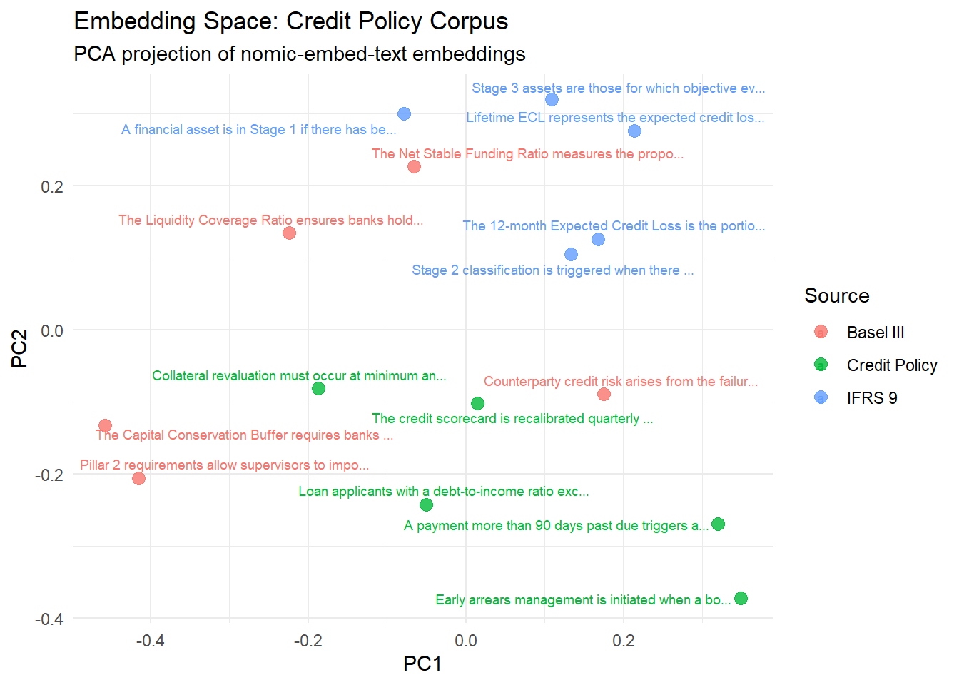
Documents from the same source seem to cluster together. The embeddings have captured domain level structure (e.g. IFRS 9 vs Basel III) even though the model was not specifically trained on financial text.
Retrieval: VSS vs BM25 vs Hybrid
ragnar supports three retrieval modes:
| Mode | Method | Description |
|---|---|---|
| VSS | Dense cosine similarity | Embedding-based cosine |
| BM25 | Sparse term frequency | TF-IDF cosine |
| Hybrid | Reciprocal Rank Fusion | Ensemble of both |
query <- "What triggers a move to Stage 2 under IFRS 9?"

# Combined (VSS + BM25)
results_hybrid <- ragnar_retrieve(store, query, top_k = 2)

# VSS only
results_vss  <- ragnar_retrieve_vss(store, query, top_k = 2)

# BM25 only
results_bm25 <- ragnar_retrieve_bm25(store, query, top_k = 2)

bind_rows(
  results_vss    |> mutate(method = "VSS",    rank = row_number()),
  results_bm25   |> mutate(method = "BM25",   rank = row_number()),
  results_hybrid |> mutate(method = "Hybrid", rank = row_number())
) |>
  select(method, rank, origin, text) |>
  arrange(method, rank)
# A tibble: 7 × 4
method rank origin text
<chr> <int> <chr> <chr>
1 BM25 1 IFRS 9 Stage 2 classification is triggered when there is …
2 BM25 2 Credit Policy A payment more than 90 days past due triggers a no…
3 Hybrid 1 IFRS 9 Stage 2 classification is triggered when there is …
4 Hybrid 2 IFRS 9 A financial asset is in Stage 1 if there has been …
5 Hybrid 3 Credit Policy A payment more than 90 days past due triggers a no…
6 VSS 1 IFRS 9 Stage 2 classification is triggered when there is …
7 VSS 2 IFRS 9 A financial asset is in Stage 1 if there has been …Hybrid retrieval tends to search for both exact keyword matches (BM25) and semantically similar chunks (VSS) whereas, VSS focuses on semantic similarity and BM25 focuses on keyword overlap.
Generating Grounded Answers with ellmer
With retrieval now working, we can use this retrieved context to generate grounded answers to specific questions. The ellmer package provides an easy to use interface for building LLM applications in R. The ragnar_register_tool_retrieve() function registers the store as a tool the LLM can call, enabling the LLM to pull relevant context before answering.
# Initialise the chat (local Ollama)
chat <- chat_ollama(
  model  = "llama3.1",
  system = "You are a credit risk analyst. Answer questions using only the
            information retrieved from the document store. If the answer is
            not in the retrieved context, say so explicitly."
)

# Register the vector store as a retrieval tool
ragnar_register_tool_retrieve(chat, store)
Comparing RAG vs No-RAG
query <- "What triggers a loan to move to Stage 2 under IFRS 9?"

# With RAG (retrieval tool registered)
answer_rag <- chat$chat(query)
Unfortunately, based on the document store, I was unable to find any
information specifically detailing what triggers a loan to move to Stage 2
under IFRS9.# Without RAG (fresh chat, no tools, no context)
chat_naive <- chat_ollama(model = "llama3.1")
answer_naive <- chat_naive$chat(query)Under IFRS 9, a loan moves from Stage 1 (measured at amortised cost) to Stage 2
when the credit risk on the loan increases due to the borrower's default or
impaired credit status.
Specifically, the criteria for moving a loan to Stage 2 are as follows:
1. **Default occurs**: The entity assumes that the debtor is unlikely to pay in
full unless the parties to the contract agree to a concession (i.e.,
restructuring). However, if the underlying contractual cash flows are not
directly affected by the default and there's no significant increase in credit
risk due to other reasons (e.g., debtors' financial difficulties), then it does
not imply that the loan should move to Stage 2.
2. **30+ days past-due payments**: The loan moves to stage 2 when the borrower
is 90 or more days past due on amounts exceeding their expected credit loss
amount from previous periods and no repayments have been made since they went
overboard.
If the initial loss event results in a significant increase of the credit
risk, the entity has grounds to recognize an allowance for expected credit
losses.tibble(
approach = c("RAG (grounded)", "No RAG (naive)"),
answer = c(answer_rag, answer_naive)
)# A tibble: 2 × 2
approach answer
<chr> <chr>
1 RAG (grounded) "Unfortunately, based on the document store, I was unable to f…
2 No RAG (naive) "Under IFRS 9, a loan moves from Stage 1 (measured at amortise…The RAG answer cites the specific IFRS 9 trigger from the corpus. The naive answer while broadly correct lacks grounding, and for certain edge cases could hallucinate and quote triggers that might not exist. Grounding the LLM with retrieved context helps keep it aligned with the source material.
Real World Application to Model Documentation
A practical use case of this setup could be to build an internal Q&A tool to query model documentation, regulatory frameworks, and policy manuals. The RAG pipeline would retrieve relevant context and generate concise answers to specific questions.
questions <- c(
  "What triggers an IFRS 9 Stage 2 migration?",
  "When is a loan classified as non-performing?",
  "What is the Capital Conservation Buffer requirement?",
  "How often is the credit scorecard recalibrated?"
)

# Helper: run a grounded query and return answer as string
ask_rag <- function(question) {
  ch <- chat_ollama(
    model  = "llama3.1",
    system = "Answer using only retrieved context. Be concise."
  )
  ragnar_register_tool_retrieve(ch, store)
  ch$chat(question)
}

# Batch Q&A as a tidy tibble
qa_results <- tibble(
  question = questions,
  answer   = purrr::map_chr(questions, ask_rag)
)
A significant increase in credit risk relative to initial recognition triggers
an IFRS 9 Stage 2 migration. This can be due to changes in macroeconomic
conditions, shifts in the applicant population, or actual payment defaults.Based on the tool call output, a loan is typically considered non-performing
when payments have stopped or been significantly delayed. Further, specific
criteria such as a payment more than 90 days past due can also trigger a
non-performing loan classification requiring full provisioning.The Capital Conservation Buffer requirement is a regulatory minimum that banks
must hold, requiring them to maintain a Common Equity Tier 1 ratio of at least
4.5% (or 7% for G-SIABS and intermediary institutions). This buffer was
introduced as part of the Basel III reforms and is intended to help banks build
stronger capital positions during times of economic stress, allowing them to
absorb potential losses without diluting shareholders' equity.The credit scorecard is recalibrated quarterly.qa_results# A tibble: 4 × 2
question answer
<chr> <chr>
1 What triggers an IFRS 9 Stage 2 migration? A significant increase i…
2 When is a loan classified as non-performing? Based on the tool call o…
3 What is the Capital Conservation Buffer requirement? The Capital Conservation…
4 How often is the credit scorecard recalibrated? The credit scorecard is …This process can be repeated as documentation is updated, ensuring the tool remains current. The local Ollama setup means this can be done without any API keys or costs, making it ideal for internal use cases.