# Load required packages
library(pso)       # For PSO implementation (provides psoptim function)
library(ggplot2)   # For data visualization
library(dplyr)     # For data manipulation and transformation
library(quantmod)  # For downloading financial data
library(tidyr)     # For reshaping data (pivot_wider, gather functions)
library(plotly)    # For creating interactive 3D visualizations
library(stringr)   # For string manipulation (used in ticker formatting)
library(purrr)     # For functional programming (reduce function)
library(slider) # For rolling calculations (rolling correlation)Portfolio Optimization Using PSO
R
Finance
Optimization
Portfolio optimization represents a critical task in investment management, where the goal involves allocating capital across different assets to maximize returns while controlling risk. This post explores how to use Particle Swarm Optimization (PSO) to perform mean-variance portfolio optimization with various constraints.
For additional information on mean-variance optimization and the CAPM model, refer to this paper.
For additional information on particle swarm optimisation, refer to this post on
Required Packages
Data Collection
The first step is to gather historical price data to calculate returns and risk metrics.
Getting Stock Tickers
This post uses stocks from the NIFTY50 index, which includes the 50 largest Indian companies by market capitalisation:
# Read ticker list from NSE (National Stock Exchange of India) website
ticker_list <- read.csv("https://raw.githubusercontent.com/royr2/datasets/refs/heads/main/ind_nifty50list.csv")

# View the first few rows
head(ticker_list[,1:3], 5)
Company.Name Industry Symbol
1 Adani Enterprises Ltd. Metals & Mining ADANIENT
2 Adani Ports and Special Economic Zone Ltd. Services ADANIPORTS
3 Apollo Hospitals Enterprise Ltd. Healthcare APOLLOHOSP
4 Asian Paints Ltd. Consumer Durables ASIANPAINT
5 Axis Bank Ltd. Financial Services AXISBANKDownloading Historical Price Data
The next step involves downloading historical price data for these stocks using the quantmod package, which provides an interface to Yahoo Finance:
# Append ".NS" to tickers for Yahoo Finance format (NS = National Stock Exchange)
tickers <- paste0(ticker_list$Symbol, ".NS")
tickers <- tickers[!tickers %in% c("ETERNAL.NS", "JIOFIN.NS", "TMPV.NS")]

# Initialize empty dataframe to store all ticker data
ticker_df <- data.frame()

# Loop through each ticker and download its historical data
for(nms in tickers){

  # Download data from Yahoo Finance
  df <- getSymbols(Symbols = nms, verbose = FALSE, auto.assign = FALSE)

  # Convert to dataframe and add ticker and date information
  df <- fortify(df)
  colnames(df) <- c("date", "open", "high", "low", "close", "volume", "adjusted")
  df$ticker <- nms

  # Append to the main dataframe
  ticker_df <- rbind(ticker_df, df)

  Sys.sleep(0.1)

}

# Reshape data to wide format with dates as rows and tickers as columns
# Remove any duplicate entries for the same date and ticker (if any)
ticker_df <- ticker_df %>%
  group_by(date, ticker) %>%
  slice(1) %>%
  ungroup()

prices_df <- pivot_wider(ticker_df, id_cols = "date", names_from = "ticker", values_from = "close")

# Remove rows with missing values to ensure complete data
prices_df <- na.omit(prices_df)

# Check the date range of our data
range(prices_df$date)
[1] "2020-08-21" "2026-04-10"# Check dimensions (number of trading days × number of stocks + date column)
dim(prices_df)[1] 1395 48Visualizing the Data
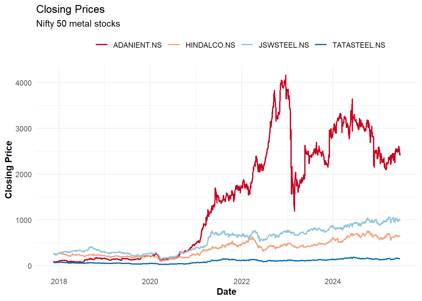
Rather than plotting raw prices, a rolling pairwise correlation chart better reveals periods of high and low co-movement between stocks — directly relevant to the diversification benefits we seek in portfolio construction.
# Extract metal stock tickers
metal_tickers <- ticker_list |>
  filter(str_detect(tolower(Industry), "metal")) |>
  mutate(ticker = paste0(Symbol, ".NS")) |>
  pull(ticker)

# Compute daily returns for metal stocks
metal_returns <- prices_df |>
  select(date, any_of(metal_tickers)) |>
  mutate(date = as.Date(date)) |>
  arrange(date) |>
  mutate(across(-date, \(x) x / lag(x) - 1)) |>
  drop_na()

dates   <- metal_returns$date
ret_mat <- as.matrix(metal_returns[, -1])

# Get all unique pairs
pairs <- combn(colnames(ret_mat), 2, simplify = FALSE)

# Rolling correlation for each pair across the data set
roll_corr <- lapply(pairs, function(pair){
  slide_dbl(1:nrow(ret_mat),
            ~ cor(ret_mat[.x, pair[1]],
                  ret_mat[.x, pair[2]]),
            .before = 60,  # Look back 60 days for rolling correlation
            .complete = TRUE)
})

# Average correlation across all pairs at each date
avg_corr <- purrr::reduce(roll_corr, `+`) / length(roll_corr)
avg_corr_df <- tibble(date = dates,
                      avg_corr = avg_corr)

# Area chart with regime shading
ggplot(avg_corr_df, aes(x = date, y = avg_corr)) +
  geom_line(linewidth = 0.7, colour = "grey30") +
  theme_minimal() +
  scale_y_continuous(limits = c(0, 1), breaks = seq(0, 1, by = 0.2)) +
  labs(
    title    = "Rolling 60-Day Average Pairwise Correlation",
    subtitle = "Nifty 50 metal stocks",
    x        = "Date",
    y        = "Average Pairwise Correlation"
  ) +
  theme(
    axis.title.x = element_text(face = "bold"),
    axis.title.y = element_text(face = "bold")
  )
The chart highlights periods of high correlation where metal stocks move together — reducing diversification benefits — and low correlation where stocks diverge, offering better risk reduction.
Calculating Returns
For portfolio optimization, we need to work with returns rather than prices. Returns better represent the investment performance and have more desirable statistical properties (like stationarity):
# Calculate daily returns for all stocks
# Formula: (Price_today / Price_yesterday) - 1
returns_df <- apply(prices_df[,-1], 2, function(vec){
  ret <- vec/lag(vec) - 1  # Simple returns calculation
  return(ret)
})

# Convert to dataframe for easier manipulation
returns_df <- as.data.frame(returns_df)

# Remove first row which contains NA values (no previous day to calculate return)
returns_df <- returns_df[-1,]

# Pre-compute average returns and covariance matrix for optimization
# These constitute key inputs to the mean-variance optimization
mean_returns <- sapply(returns_df, mean)  # Expected returns
cov_mat <- cov(returns_df)  # Risk (covariance) matrix
The mean returns represent expectations for each asset’s performance, while the covariance matrix captures both the individual volatilities and the relationships between assets. These serve as inputs to the optimization process.
Portfolio Optimization Framework
Objective Function
In mean-variance optimisation the objective function, which defines the optimization target balances three key components:
- Expected returns (reward): The weighted average of expected returns for each asset
- Portfolio variance (risk): A measure of the portfolio’s volatility, calculated using the covariance matrix
- Risk aversion parameter: Controls the trade-off between risk and return (higher values prioritize risk reduction)
The implementation also incorporates constraints through penalty terms:
obj_func <- function(wts,
                     risk_av = 10,  # Risk aversion parameter
                     lambda1 = 10,  # Penalty weight for full investment constraint
                     lambda2 = 1e2,  # Reserved for additional constraints
                     ret_vec, cov_mat){

  # Calculate expected portfolio return (weighted average of asset returns)
  port_returns <- ret_vec %*% wts

  # Calculate portfolio risk (quadratic form using covariance matrix)
  port_risk <- t(wts) %*% cov_mat %*% wts

  # Mean-variance utility function: return - risk_aversion * risk
  # This is the core Markowitz portfolio optimization formula
  obj <- port_returns - risk_av * port_risk

  # Add penalty for violating the full investment constraint (sum of weights = 1)
  # The squared term ensures the penalty increases quadratically with violation size
  obj <- obj - lambda1 * (sum(wts) - 1)^2
  # Return negative value since PSO minimizes by default, but the goal is to maximize
  # the objective (higher returns, lower risk)
  return(-obj)
}
This objective function implements the classic mean-variance utility with a quadratic penalty for the full investment constraint. The risk aversion parameter allows us to move along the efficient frontier to find portfolios with different risk-return profiles.
Two-Asset Example
Before tackling the full portfolio optimization problem, this section begins with a simple two-asset example. This approach helps visualize how PSO works and validates the methodology:
# Use only the first two assets for this example
# Calculate their average returns and covariance matrix
mean_returns_small <- apply(returns_df[,1:2], 2, mean)
cov_mat_small <- cov(returns_df[,1:2])

# Define a custom PSO optimizer function to track the optimization process
pso_optim <- function(obj_func,
                      c1 = 0.05,      # Cognitive parameter (personal best influence)
                      c2 = 0.05,      # Social parameter (global best influence)
                      w = 0.8,        # Inertia weight (controls momentum)
                      init_fact = 0.1, # Initial velocity factor
                      n_particles = 20, # Number of particles in the swarm
                      n_dim = 2,       # Dimensionality (number of assets)
                      n_iter = 50,     # Maximum iterations
                      upper = 1,       # Upper bound for weights
                      lower = 0,       # Lower bound for weights (no short selling)
                      n_avg = 10,      # Number of iterations for averaging
                      ...){

  # Initialize particle positions randomly within bounds
  X <- matrix(runif(n_particles * n_dim), nrow = n_particles)
  X <- X * (upper - lower) + lower  # Scale to fit within bounds

  # Initialize particle velocities (movement speeds)
  dX <- matrix(runif(n_particles * n_dim) * init_fact, ncol = n_dim)
  dX <- dX * (upper - lower) + lower

  # Initialize personal best positions and objective values
  pbest <- X  # Each particle's best position so far
  pbest_obj <- apply(X, 1, obj_func, ...)  # Objective value at personal best

  # Initialize global best position and objective value
  gbest <- pbest[which.min(pbest_obj),]  # Best position across all particles
  gbest_obj <- min(pbest_obj)  # Best objective value found

  # Store initial positions for visualization
  loc_df <- data.frame(X, iter = 0, obj = pbest_obj)
  iter <- 1

  # Main PSO loop
  while(iter < n_iter){

    # Update velocities using PSO formula:
    # New velocity = inertia + cognitive component + social component
    dX <- w * dX +                         # Inertia (continue in same direction)
      c1*runif(1)*(pbest - X) +        # Pull toward personal best
      c2*runif(1)*t(gbest - t(X))      # Pull toward global best

    # Update positions based on velocities
    X <- X + dX

    # Evaluate objective function at new positions
    obj <- apply(X, 1, obj_func, ...)

    # Update personal bests if new positions are better
    idx <- which(obj <= pbest_obj)
    pbest[idx,] <- X[idx,]
    pbest_obj[idx] <- obj[idx]

    # Update global best if a better solution is found
    idx <- which.min(pbest_obj)
    gbest <- pbest[idx,]
    gbest_obj <- min(pbest_obj)

    # Store current state for visualization
    iter <- iter + 1
    loc_df <- rbind(loc_df, data.frame(X, iter = iter, obj = pbest_obj))
  }

  # Return optimization results
  lst <- list(X = loc_df,          # All particle positions throughout optimization
              obj = gbest_obj,     # Best objective value found
              obj_loc = gbest)     # Weights that achieved the best objective
  return(lst)
}

# Run the optimization for our two-asset portfolio
out <- pso_optim(obj_func,
                 ret_vec = mean_returns_small,  # Expected returns
                 cov_mat = cov_mat_small,       # Covariance matrix
                 lambda1 = 10, risk_av = 100,    # Constraint and risk parameters
                 n_particles = 100,              # Use 100 particles for better coverage
                 n_dim = 2,                      # Two-asset portfolio
                 n_iter = 200,                   # Run for 200 iterations
                 upper = 1, lower = 0,           # Bounds for weights
                 c1 = 0.02, c2 = 0.02,           # Lower influence parameters for stability
                 w = 0.05, init_fact = 0.01)     # Low inertia for better convergence

# Verify that the weights sum to approximately 1 (full investment constraint)
sum(out$obj_loc)
[1] 0.9988184In this implementation, the tracking of all particle movements throughout the optimization process occurs. This enables visualization of how the swarm converges toward the optimal solution.
Visualizing the Optimization Process
One advantage of starting with a two-asset example is the ability to visualize the entire search space and observe how the PSO algorithm explores it. The following creates a 3D visualization of the objective function landscape and the path each particle took during optimization:
# Create a fine grid of points covering the feasible region (all possible weight combinations)
grid <- expand.grid(x = seq(0, 1, by = 0.01),  # First asset weight from 0 to 1
                    y = seq(0, 1, by = 0.01))   # Second asset weight from 0 to 1

# Evaluate the objective function at each grid point to create the landscape
grid$obj <- apply(grid, 1, obj_func,
                  ret_vec = mean_returns_small,
                  cov_mat = cov_mat_small,
                  lambda1 = 10, risk_av = 100)

# Create an interactive 3D plot showing both the objective function surface
# and the particle trajectories throughout the optimization
p <- plot_ly() %>%
  # Add the objective function surface as a mesh
  add_mesh(data = grid, x = ~x, y = ~y, z = ~obj,
           inherit = FALSE, color = "red") %>%

  # Add particles as markers, colored by iteration to show progression
  add_markers(data = out$X, x = ~X1, y = ~X2, z = ~obj,
              color = ~ iter, inherit = FALSE,
              marker = list(size = 2))
This visualization demonstrates:
- The objective function landscape as a 3D surface
- The particles (small dots) exploring the search space
- How the swarm converges toward the optimal solution over iterations (color gradient)
The concentration of particles in certain regions indicates where the algorithm found promising solutions. The global best solution represents where the particles ultimately converge.
Multi-Asset Portfolio Optimization
To scale the problem to multiple assets, instead of using the custom PSO implementation, this section leverages the psoptim function from the pso package:
# Get the number of stocks in the dataset
n_stocks <- ncol(returns_df)

# Run the PSO optimization for the full portfolio
opt <- psoptim(
  # Initial particle positions (starting with equal weights)
  par = rep(0, n_stocks),

  # Objective function to minimize
  fn = obj_func,

  # Pass the expected returns and covariance matrix
  ret_vec = mean_returns,
  cov_mat = cov_mat,

  # Set constraint parameters
  lambda1 = 10,  # Weight for full investment constraint
  risk_av = 1000,  # Higher risk aversion for a more conservative portfolio

  # Set bounds for weights (no short selling allowed)
  lower = rep(0, n_stocks),
  upper = rep(1, n_stocks),

  # Configure the PSO algorithm
  control = list(
    maxit = 200,          # Maximum iterations
    s = 100,               # Swarm size (number of particles)
    maxit.stagnate = 500   # Stop if no improvement after this many iterations
  )
)

# Calculate and display the expected return of the optimized portfolio
paste("Portfolio returns:", round(opt$par %*% mean_returns, 5))
[1] "Portfolio returns: 0.00053"# Calculate and display the standard deviation (risk) of the optimized portfolio
paste("Portfolio Std dev:", round(sqrt(opt$par %*% cov_mat %*% opt$par), 5))[1] "Portfolio Std dev: 0.00753"# Verify that the weights sum to approximately 1 (full investment constraint)
sum(opt$par)[1] 0.9934328Adding Tracking Error Constraint
Tracking error measures how closely a portfolio follows a benchmark.
# Define benchmark portfolio (equally weighted across all stocks)
bench_wts <- rep(1/n_stocks, n_stocks)

# Calculate the time series of benchmark returns
bench_returns <- as.matrix(returns_df) %*% t(t(bench_wts))

# Create a new objective function that includes tracking error
obj_func_TE <- function(wts,
                        risk_av = 10,     # Risk aversion parameter
                        lambda1 = 10,    # Full investment constraint weight
                        lambda2 = 50,    # Tracking error constraint weight
                        ret_vec, cov_mat){

  # Calculate portfolio metrics
  port_returns <- ret_vec %*% wts                      # Expected portfolio return
  port_risk <- t(wts) %*% cov_mat %*% wts             # Portfolio variance
  port_returns_ts <- as.matrix(returns_df) %*% t(t(wts))  # Time series of portfolio returns

  # Original mean-variance objective
  obj <- port_returns - risk_av * port_risk

  # Full investment constraint (weights sum to 1)
  obj <- obj - lambda1 * (sum(wts) - 1)^2

  # Tracking error constraint (penalize deviation from benchmark)
  # Tracking error is measured as the standard deviation of the difference
  # between portfolio returns and benchmark returns
  obj <- obj - lambda2 * sd(port_returns_ts - bench_returns)

  return(-obj)  # Return negative for minimization
}

# Run optimization with the tracking error constraint
opt <- psoptim(
  # Initial particle positions
  par = rep(0, n_stocks),

  # Use our new objective function with tracking error
  fn = obj_func_TE,

  # Pass the expected returns and covariance matrix
  ret_vec = mean_returns,
  cov_mat = cov_mat,

  # Set constraint parameters
  lambda1 = 10,    # Weight for full investment constraint
  risk_av = 1000,  # Risk aversion parameter

  # Set bounds for weights
  lower = rep(0, n_stocks),
  upper = rep(1, n_stocks),

  # Configure the PSO algorithm
  control = list(
    maxit = 200,          # Maximum iterations
    s = 100,               # Swarm size
    maxit.stagnate = 500   # Stop if no improvement after this many iterations
  )
)

# Calculate and display the expected return of the optimized portfolio
paste("Portfolio returns:", round(opt$par %*% mean_returns, 5))
[1] "Portfolio returns: 9e-04"# Calculate and display the standard deviation (risk) of the optimized portfolio
paste("Portfolio Std dev:", round(sqrt(opt$par %*% cov_mat %*% opt$par), 5))[1] "Portfolio Std dev: 0.00909"# Verify that the weights sum to approximately 1
sum(opt$par)[1] 0.9910437Adding the tracking error constraint, not only balances risk and return but also tracks the performance of an equally-weighted benchmark. The lambda2 parameter controls the closeness of benchmark tracking - higher values result in portfolios that more closely resemble the benchmark.
Advantages and Limitations of PSO
Advantages:
Flexibility: PSO can handle non-convex, non-differentiable objective functions, making it suitable for complex portfolio constraints that traditional optimizers struggle with
Simplicity: The algorithm is intuitive and relatively easy to implement compared to other global optimization techniques
Constraints: Various constraints can be easily incorporated through penalty functions without reformulating the entire problem
Global Search: PSO explores the search space more thoroughly and is less likely to get stuck in local optima compared to gradient-based methods
Parallelization: The algorithm is naturally parallelizable, as particles can be evaluated independently
Limitations:
Variability: Results can vary between runs due to the stochastic nature of the algorithm, potentially leading to inconsistent portfolio recommendations
Parameter Tuning: Performance significantly depends on parameters like inertia weight and acceleration coefficients, which may require careful tuning
Convergence: There’s no mathematical guarantee of convergence to the global optimum, unlike some convex optimization methods
Computational Cost: Can be computationally intensive for high-dimensional problems with many assets
Constraint Handling: While flexible, the penalty function approach may not always satisfy constraints exactly
Practical Applications
PSO-based portfolio optimization proves particularly valuable in scenarios where:
- Traditional quadratic programming approaches fail due to complex constraints
- The objective function includes non-linear terms like higher moments (skewness, kurtosis)
- Multiple competing objectives need to be balanced
- The portfolio needs to satisfy regulatory or client-specific constraints
The approach demonstrated in this post can be extended to include additional constraints such as:
- Sector or industry exposure limits
- Maximum position sizes
- Turnover or transaction cost constraints
- Risk factor exposures and limits
- Cardinality constraints (limiting the number of assets)